Ch03 Linear Regression Lab
The material in this file is adapted from the Jupyter notebooks in the resources accompanying the book An Introduction to Statistical Learning by James, Witten, Hastie & Tibshirani under this LICENSE.
Importing packages
We import our standard libraries at this top level.
import numpy as np
import polars as pl
import pandas as pd
from matplotlib.pyplot import subplots
New imports
Throughout this lab we will introduce new functions and libraries. However, we will import them here to emphasize these are the new code objects in this lab. Keeping imports near the top of a notebook makes the code more readable, since scanning the first few lines tells us what libraries are used.
import statsmodels.api as sm
We will provide relevant details about the functions below as they are needed.
Besides importing whole modules, it is also possible to import only a few items
from a given module. This will help keep the namespace clean. We will use a few
specific objects from the statsmodels package which we import here.
from statsmodels.stats.anova import anova_lm
from statsmodels.stats.outliers_influence import \
    variance_inflation_factor as VIF
As one of the import statements above is quite a long line, we inserted
a line break \ to ease readability.
We will also use some functions written for the labs in this book in the
ISLP package.
from ISLP.models import ModelSpec as MS
from ISLP.models import poly, summarize
Inspecting Objects and Namespaces
The function dir() provides a list of objects in a namespace.
dir()
['In',
 'MS',
 'Out',
 'VIF',
 '_',
 '__',
 '___',
 '__builtin__',
 '__builtins__',
 '__doc__',
 '__loader__',
 '__name__',
 '__package__',
 '__spec__',
 '_dh',
 '_i',
 '_i1',
 '_i2',
 '_i3',
 '_i4',
 '_i5',
 '_ih',
 '_ii',
 '_iii',
 '_oh',
 'anova_lm',
 'exit',
 'get_ipython',
 'np',
 'open',
 'pd',
 'pl',
 'poly',
 'quit',
 'sm',
 'subplots',
 'summarize']
This shows you everything that Python can find at the top level. There
are certain objects like __builtins__ that contain references to
built-in functions like print().
Every python object has its own notion of namespace, also accessible
with dir(). This will include both the attributes of the object as
well as any methods associated with it. For instance, we see 'sum' in
the listing for an array.
A = np.array([3,5,11])
dir(A)
['T',
 '__abs__',
 '__add__',
 '__and__',
 '__array__',
 '__array_finalize__',
 '__array_function__',
 '__array_interface__',
 '__array_namespace__',
 '__array_priority__',
 '__array_struct__',
 '__array_ufunc__',
 '__array_wrap__',
 '__bool__',
 '__buffer__',
 '__class__',
 '__class_getitem__',
 '__complex__',
 '__contains__',
 '__copy__',
 '__deepcopy__',
 '__delattr__',
 '__delitem__',
 '__dir__',
 '__divmod__',
 '__dlpack__',
 '__dlpack_device__',
 '__doc__',
 '__eq__',
 '__float__',
 '__floordiv__',
 '__format__',
 '__ge__',
 '__getattribute__',
 '__getitem__',
 '__getstate__',
 '__gt__',
 '__hash__',
 '__iadd__',
 '__iand__',
 '__ifloordiv__',
 '__ilshift__',
 '__imatmul__',
 '__imod__',
 '__imul__',
 '__index__',
 '__init__',
 '__init_subclass__',
 '__int__',
 '__invert__',
 '__ior__',
 '__ipow__',
 '__irshift__',
 '__isub__',
 '__iter__',
 '__itruediv__',
 '__ixor__',
 '__le__',
 '__len__',
 '__lshift__',
 '__lt__',
 '__matmul__',
 '__mod__',
 '__mul__',
 '__ne__',
 '__neg__',
 '__new__',
 '__or__',
 '__pos__',
 '__pow__',
 '__radd__',
 '__rand__',
 '__rdivmod__',
 '__reduce__',
 '__reduce_ex__',
 '__repr__',
 '__rfloordiv__',
 '__rlshift__',
 '__rmatmul__',
 '__rmod__',
 '__rmul__',
 '__ror__',
 '__rpow__',
 '__rrshift__',
 '__rshift__',
 '__rsub__',
 '__rtruediv__',
 '__rxor__',
 '__setattr__',
 '__setitem__',
 '__setstate__',
 '__sizeof__',
 '__str__',
 '__sub__',
 '__subclasshook__',
 '__truediv__',
 '__xor__',
 '_set_dtype',
 '_set_shape',
 'all',
 'any',
 'argmax',
 'argmin',
 'argpartition',
 'argsort',
 'astype',
 'base',
 'byteswap',
 'choose',
 'clip',
 'compress',
 'conj',
 'conjugate',
 'copy',
 'ctypes',
 'cumprod',
 'cumsum',
 'data',
 'device',
 'diagonal',
 'dot',
 'dtype',
 'dump',
 'dumps',
 'fill',
 'flags',
 'flat',
 'flatten',
 'getfield',
 'imag',
 'item',
 'itemsize',
 'mT',
 'max',
 'mean',
 'min',
 'nbytes',
 'ndim',
 'nonzero',
 'partition',
 'prod',
 'put',
 'ravel',
 'real',
 'repeat',
 'reshape',
 'resize',
 'round',
 'searchsorted',
 'setfield',
 'setflags',
 'shape',
 'size',
 'sort',
 'squeeze',
 'std',
 'strides',
 'sum',
 'swapaxes',
 'take',
 'to_device',
 'tobytes',
 'tofile',
 'tolist',
 'trace',
 'transpose',
 'var',
 'view']
This indicates that the object A.sum exists. In this case it is a method that
can be used to compute the sum of the array A as can be seen by typing A.sum?.
A.sum()
np.int64(19)
Simple Linear Regression
In this section we will construct model matrices (also called design matrices)
using the ModelSpec() transform from ISLP.models.
We will use the Boston housing data set, which is contained in the ISLP
package. The Boston dataset records medv (median house value) for \(506\)
neighborhoods around Boston. We will build a regression model to predict medv
using \(13\) predictors such as rm (average number of rooms per house), age
(proportion of owner-occupied units built prior to 1940), and lstat (percent of
households with low socioeconomic status). We will use statsmodels for this
task, a Python package that implements several commonly used regression
methods.
We have included a simple loading function load_data() in the ISLP
package:
from pathlib import Path


def load_data(dataset):
    data_dir = Path(
        "/home/bon/projects/auc/courses/ml/website/data/"
        "ALL CSV FILES - 2nd Edition"
    )
    data_file = dataset + ".csv"
    return pl.read_csv(data_dir / data_file)


Boston = load_data("Boston")
Boston.columns
['',
 'crim',
 'zn',
 'indus',
 'chas',
 'nox',
 'rm',
 'age',
 'dis',
 'rad',
 'tax',
 'ptratio',
 'lstat',
 'medv']
Type Boston? to find out more about these data.
We start by using the sm.OLS() function to fit a simple linear regression
model. Our response will be medv and lstat will be the single predictor. For
this model, we can create the model matrix by hand.
X = pl.DataFrame({'intercept': np.ones(Boston.shape[0]),
                  'lstat': Boston['lstat']})
X[:4]
shape: (4, 2)
┌───────────┬───────┐
│ intercept ┆ lstat │
│ ---       ┆ ---   │
│ f64       ┆ f64   │
╞═══════════╪═══════╡
│ 1.0       ┆ 4.98  │
│ 1.0       ┆ 9.14  │
│ 1.0       ┆ 4.03  │
│ 1.0       ┆ 2.94  │
└───────────┴───────┘
We extract the response, and fit the model.
y = Boston['medv']
model = sm.OLS(y, X)
results = model.fit()
Note that sm.OLS() does not fit the model; it specifies the model, and then
model.fit() does the actual fitting.
Our ISLP function summarize() produces a simple table of the parameter
estimates, their standard errors, t-statistics and p-values. The function takes
a single argument, such as the object results returned here by the fit method,
and returns such a summary.
summarize(results)
              coef  std err       t  P>|t|
intercept  34.5538    0.563  61.415    0.0
lstat      -0.9500    0.039 -24.528    0.0
Before we describe other methods for working with fitted models, we outline a
more useful and general framework for constructing a model matrix~=X=. ###
Using Transformations: Fit and Transform Our model above has a single
predictor, and constructing X was straightforward. In practice we often fit
models with more than one predictor, typically selected from an array or data
frame. We may wish to introduce transformations to the variables before fitting
the model, specify interactions between variables, and expand some particular
variables into sets of variables (e.g. polynomials). The sklearn package has a
particular notion for this type of task: a transform. A transform is an object
that is created with some parameters as arguments. The object has two main
methods: fit() and transform().
We provide a general approach for specifying models and constructing the model
matrix through the transform ModelSpec() in the ISLP library. ModelSpec()
(renamed MS() in the preamble) creates a transform object, and then a pair of
methods transform() and fit() are used to construct a corresponding model
matrix.
We first describe this process for our simple regression model using a single
predictor lstat in the Boston data frame, but will use it repeatedly in more
complex tasks in this and other labs in this book. In our case the transform is
created by the expression design = MS(['lstat']).
The fit() method takes the original array and may do some initial computations
on it, as specified in the transform object. For example, it may compute means
and standard deviations for centering and scaling. The transform() method
applies the fitted transformation to the array of data, and produces the model
matrix.
Since design.fit takes a Numpy data frame, we need to convert Boston before
passing it.
design = MS(["lstat"])
Boston = Boston.to_pandas()
design = design.fit(Boston)
X = design.transform(Boston)
X[:4]
   intercept  lstat
0        1.0   4.98
1        1.0   9.14
2        1.0   4.03
3        1.0   2.94
In this simple case, the fit() method does very little; it simply checks that
the variable 'lstat' specified in design exists in Boston. Then transform()
constructs the model matrix with two columns: an intercept and the variable
lstat.
These two operations can be combined with the fit_transform() method.
design = MS(['lstat'])
X = design.fit_transform(Boston)
X[:4]
   intercept  lstat
0        1.0   4.98
1        1.0   9.14
2        1.0   4.03
3        1.0   2.94
Note that, as in the previous code chunk when the two steps were done
separately, the design object is changed as a result of the fit() operation.
The power of this pipeline will become clearer when we fit more complex models
that involve interactions and transformations.
Let's return to our fitted regression model. The object results has several
methods that can be used for inference. We already presented a function
summarize() for showing the essentials of the fit. For a full and somewhat
exhaustive summary of the fit, we can use the summary() method.
results.summary()
<class 'statsmodels.iolib.summary.Summary'>
"""
                            OLS Regression Results
==============================================================================
Dep. Variable:                   medv   R-squared:                       0.544
Model:                            OLS   Adj. R-squared:                  0.543
Method:                 Least Squares   F-statistic:                     601.6
Date:                Thu, 17 Sep 2026   Prob (F-statistic):           5.08e-88
Time:                        13:19:38   Log-Likelihood:                -1641.5
No. Observations:                 506   AIC:                             3287.
Df Residuals:                     504   BIC:                             3295.
Df Model:                           1
Covariance Type:            nonrobust
==============================================================================
                 coef    std err          t      P>|t|      [0.025      0.975]
------------------------------------------------------------------------------
intercept     34.5538      0.563     61.415      0.000      33.448      35.659
lstat         -0.9500      0.039    -24.528      0.000      -1.026      -0.874
==============================================================================
Omnibus:                      137.043   Durbin-Watson:                   0.892
Prob(Omnibus):                  0.000   Jarque-Bera (JB):              291.373
Skew:                           1.453   Prob(JB):                     5.36e-64
Kurtosis:                       5.319   Cond. No.                         29.7
==============================================================================

Notes:
[1] Standard Errors assume that the covariance matrix of the errors is correctly specified.
"""
The fitted coefficients can also be retrieved as the params attribute of
results.
results.params
intercept    34.553841
lstat        -0.950049
dtype: float64
The get_prediction() method can be used to obtain predictions, and
produce confidence intervals and prediction intervals for the prediction
of medv for given values of lstat.
We first create a new data frame, in this case containing only the
variable lstat, with the values for this variable at which we wish to
make predictions. We then use the transform() method of design to
create the corresponding model matrix.
new_df = pd.DataFrame({'lstat':[5, 10, 15]})
newX = design.transform(new_df)
newX
   intercept  lstat
0        1.0      5
1        1.0     10
2        1.0     15
Next we compute the predictions at newX, and view them by extracting
the predicted_mean attribute.
new_predictions = results.get_prediction(newX);
new_predictions.predicted_mean
array([29.80359411, 25.05334734, 20.30310057])
We can produce confidence intervals for the predicted values.
new_predictions.conf_int(alpha=0.05)
array([[29.00741194, 30.59977628],
       [24.47413202, 25.63256267],
       [19.73158815, 20.87461299]])
Prediction intervals are computed by setting obs=True:
new_predictions.conf_int(obs=True, alpha=0.05)
array([[17.56567478, 42.04151344],
       [12.82762635, 37.27906833],
       [ 8.0777421 , 32.52845905]])
For instance, the 95% confidence interval associated with an lstat
value of 10 is (24.47, 25.63), and the 95% prediction interval is
(12.82, 37.28). As expected, the confidence and prediction intervals are
centered around the same point (a predicted value of 25.05 for medv
when lstat equals 10), but the latter are substantially wider.
Next we will plot medv and lstat using DataFrame.plot.scatter(),
plot.scatter(), plot.slashslashscatter() and wish to
add the regression line to the resulting plot.
Defining Functions
While there is a function within the ISLP package that adds a line to
an existing plot, we take this opportunity to define our first function
to do so.
def abline(ax, b, m):
    "Add a line with slope m and intercept b to ax"
    xlim = ax.get_xlim()
    ylim = [m * xlim[0] + b, m * xlim[1] + b]
    ax.plot(xlim, ylim)
A few things are illustrated above. First we see the syntax for defining
a function: def funcname(...). The function has arguments ax, b, m
where ax is an axis object for an existing plot, b is the intercept
and m is the slope of the desired line. Other plotting options can be
passed on to ax.plot by including additional optional arguments as
follows:
def abline(ax, b, m, *args, **kwargs):
    "Add a line with slope m and intercept b to ax"
    xlim = ax.get_xlim()
    ylim = [m * xlim[0] + b, m * xlim[1] + b]
    ax.plot(xlim, ylim, *args, **kwargs)
The addition of *args allows any number of non-named arguments to abline, while
**kwargs allows any number of named arguments (such as linewidth=3) to abline.
In our function, we pass these arguments verbatim to ax.plot above. Readers
interested in learning more about functions are referred to the section on
defining functions in docs.python.org/tutorial.
Let's use our new function to add this regression line to a plot of medv
vs. lstat.
plotfile = "../images/medv.png"
ax = Boston.plot.scatter("lstat", "medv")
abline(
    ax,
    results.params["intercept"],
    results.params["lstat"],
    "r--",
    linewidth=3,
)
ax.figure.savefig(plotfile)
plotfile
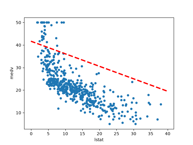
Thus, the final call to ax.plot() is ax.plot(xlim, ylim, 'r--', linewidth=3).
We have used the argument 'r--' to produce a red dashed line, and added an
argument to make it of width 3. There is some evidence for non-linearity in the
relationship between lstat and medv. We will explore this issue later in this
lab.
As mentioned above, there is an existing function to add a line to a plot —
ax.axline() — but knowing how to write such functions empowers us to create
more expressive displays.
Next we examine some diagnostic plots, several of which were discussed in
Section 3.3.3. We can find the fitted values and residuals of the fit as
attributes of the results object. Various influence measures describing the
regression model are computed with the get_influence() method. As we will not
use the fig component returned as the first value from subplots(), we simply
capture the second returned value in ax below.
plotfile = "../images/fitted_values.png"
ax = subplots(figsize=(8, 8))[1]
ax.scatter(results.fittedvalues, results.resid)
ax.set_xlabel("Fitted value")
ax.set_ylabel("Residual")
ax.axhline(0, c="k", ls="--")
ax.figure.savefig(plotfile)
plotfile
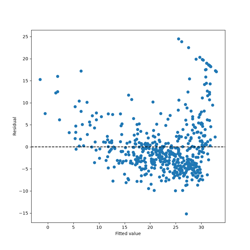
We add a horizontal line at 0 for reference using the ax.axhline()
method, indicating it should be black (c'k') and have a dashed
linestyle (=ls'–'=).
On the basis of the residual plot, there is some evidence of
non-linearity. Leverage statistics can be computed for any number of
predictors using the hat_matrix_diag attribute of the value returned
by the get_influence() method.
plotfile = "../images/leverage.png"
infl = results.get_influence()
ax = subplots(figsize=(8, 8))[1]
ax.scatter(np.arange(X.shape[0]), infl.hat_matrix_diag)
ax.set_xlabel("Index")
ax.set_ylabel("Leverage")
ax.figure.savefig(plotfile)
plotfile
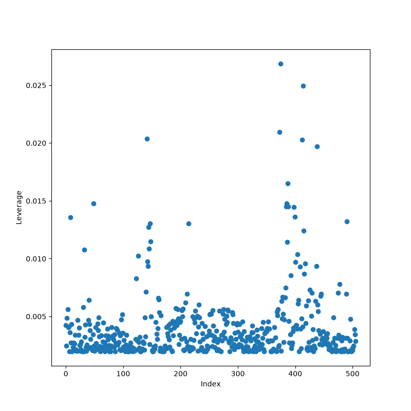
np.argmax(infl.hat_matrix_diag)
np.int64(374)
The np.argmax() function identifies the index of the largest element
of an array, optionally computed over an axis of the array. In this
case, we maximized over the entire array to determine which observation
has the largest leverage statistic.
Multiple Linear Regression
In order to fit a multiple linear regression model using least squares,
we again use the ModelSpec() transform to construct the required model
matrix and response. The arguments to ModelSpec() can be quite
general, but in this case a list of column names suffice. We consider a
fit here with the two variables lstat and age.
X = MS(['lstat', 'age']).fit_transform(Boston)
model1 = sm.OLS(y, X)
results1 = model1.fit()
summarize(results1)
              coef  std err       t  P>|t|
intercept  33.2228    0.731  45.458  0.000
lstat      -1.0321    0.048 -21.416  0.000
age         0.0345    0.012   2.826  0.005
Notice how we have compacted the first line into a succinct expression
describing the construction of X.
The Boston data set contains 12 variables, and so it would be
cumbersome to have to type all of these in order to perform a regression
using all of the predictors. Instead, we can use the following
short-hand:\definelongblankMR{columns.drop()}{columns.slashslashdrop()}
terms = Boston.columns.drop('medv')
terms
Index(['', 'crim', 'zn', 'indus', 'chas', 'nox', 'rm', 'age', 'dis', 'rad',
       'tax', 'ptratio', 'lstat'],
      dtype='str')
We can now fit the model with all the variables in terms using the
same model matrix builder.
X = MS(terms).fit_transform(Boston)
model = sm.OLS(y, X)
results = model.fit()
summarize(results)
              coef  std err       t  P>|t|
intercept  41.6430    4.934   8.439  0.000
NaN        -0.0024    0.002  -1.154  0.249
crim       -0.1222    0.033  -3.703  0.000
zn          0.0485    0.014   3.480  0.001
indus       0.0128    0.062   0.207  0.836
chas        2.8585    0.870   3.286  0.001
nox       -18.5465    3.854  -4.812  0.000
rm          3.6856    0.421   8.759  0.000
age         0.0011    0.014   0.081  0.935
dis        -1.5079    0.202  -7.461  0.000
rad         0.3075    0.069   4.476  0.000
tax        -0.0120    0.004  -3.112  0.002
ptratio    -0.9329    0.132  -7.055  0.000
lstat      -0.5535    0.051 -10.926  0.000
What if we would like to perform a regression using all of the variables
but one? For example, in the above regression output, age has a high
\(p\)-value. So we may wish to run a regression excluding this
predictor. The following syntax results in a regression using all
predictors except age.
minus_age = Boston.columns.drop(['medv', 'age'])
Xma = MS(minus_age).fit_transform(Boston)
model1 = sm.OLS(y, Xma)
summarize(model1.fit())
              coef  std err       t  P>|t|
intercept  41.6160    4.918   8.461  0.000
NaN        -0.0025    0.002  -1.184  0.237
crim       -0.1222    0.033  -3.707  0.000
zn          0.0484    0.014   3.494  0.001
indus       0.0128    0.062   0.207  0.836
chas        2.8625    0.868   3.299  0.001
nox       -18.4633    3.712  -4.974  0.000
rm          3.6927    0.411   8.981  0.000
dis        -1.5128    0.193  -7.856  0.000
rad         0.3072    0.069   4.481  0.000
tax        -0.0120    0.004  -3.115  0.002
ptratio    -0.9320    0.132  -7.081  0.000
lstat      -0.5522    0.048 -11.547  0.000
Multivariate Goodness of Fit
We can access the individual components of results by name (dir(results) shows
us what is available). Hence results.rsquared gives us the \(R^2\), and
np.sqrt(results.scale) gives us the RSE.
Variance inflation factors (section 3.3.3) are sometimes useful to assess the effect of collinearity in the model matrix of a regression model. We will compute the VIFs in our multiple regression fit, and use the opportunity to introduce the idea of list comprehension.
List Comprehension
Often we encounter a sequence of objects which we would like to transform for
some other task. Below, we compute the VIF for each feature in our X matrix and
produce a data frame whose index agrees with the columns of X. The notion of
list comprehension can often make such a task easier.
List comprehensions are simple and powerful ways to form lists of Python
objects. The language also supports dictionary and generator comprehension,
though these are beyond our scope here. Let's look at an example. We compute
the VIF for each of the variables in the model matrix X, using the function
variance_inflation_factor().
vals = [VIF(X, i) for i in range(1, X.shape[1])]
vif = pd.DataFrame({"vif": vals}, index=X.columns[1:])
vif
              vif
         2.075206
crim     1.768234
zn       2.319982
indus    3.987493
chas     1.071531
nox      4.378998
rm       1.918686
age      3.170744
dis      3.975430
rad      7.852686
tax      9.235799
ptratio  1.798726
lstat    2.872657
The function VIF() takes two arguments: a dataframe or array, and a
variable column index. In the code above we call VIF() on the fly for
all columns in X.
We have excluded column 0 above (the intercept), which is not of
interest. In this case the VIFs are not that exciting.
The object vals above could have been constructed with the following
for loop:
vals = []
for i in range(1, X.values.shape[1]):
    vals.append(VIF(X.values, i))
vals
[np.float64(2.075206317506886),
 np.float64(1.7682344258256653),
 np.float64(2.319982038608995),
 np.float64(3.987492972404629),
 np.float64(1.0715314397805453),
 np.float64(4.378997560684944),
 np.float64(1.9186859673931531),
 np.float64(3.1707442257953824),
 np.float64(3.975429618006906),
 np.float64(7.852685735148857),
 np.float64(9.235799401951617),
 np.float64(1.7987264759517363),
 np.float64(2.8726569830400472)]
List comprehension allows us to perform such repetitive operations in a more straightforward way.
Interaction Terms
It is easy to include interaction terms in a linear model using ModelSpec().
Including a tuple ("lstat","age") tells the model matrix builder to include an
interaction term between lstat and age.
X = MS(["lstat", "age", ("lstat", "age")]).fit_transform(Boston)
model2 = sm.OLS(y, X)
summarize(model2.fit())
              coef  std err       t  P>|t|
intercept  36.0885    1.470  24.553  0.000
lstat      -1.3921    0.167  -8.313  0.000
age        -0.0007    0.020  -0.036  0.971
lstat:age   0.0042    0.002   2.244  0.025
Non-linear Transformations of the Predictors
The model matrix builder can include terms beyond just column names and
interactions. For instance, the poly() function supplied in ISLP
specifies that columns representing polynomial functions of its first
argument are added to the model matrix.
X = MS([poly('lstat', degree=2), 'age']).fit_transform(Boston)
model3 = sm.OLS(y, X)
results3 = model3.fit()
summarize(results3)
                              coef  std err       t  P>|t|
intercept                  17.7151    0.781  22.681    0.0
poly(lstat, degree=2)[0] -179.2279    6.733 -26.620    0.0
poly(lstat, degree=2)[1]   72.9908    5.482  13.315    0.0
age                         0.0703    0.011   6.471    0.0
The effectively zero p-value associated with the quadratic term (i.e. the third row above) suggests that it leads to an improved model.
By default, poly() creates a basis matrix for inclusion in the model
matrix whose columns are orthogonal polynomials, which are designed
for stable least squares computations. {Actually, poly() is a wrapper
for the workhorse and standalone function Poly() that does the work in
building the model matrix.} Alternatively, had we included an argument
raw=True in the above call to poly(), the basis matrix would consist
simply of lstat and lstat**2. Since either of these bases represent
quadratic polynomials, the fitted values would not change in this case,
just the polynomial coefficients. Also by default, the columns created
by poly() do not include an intercept column as that is automatically
added by MS().
We use the anova_lm() function to further quantify the extent to which
the quadratic fit is superior to the linear fit.
anova_lm(results1, results3)
   df_resid           ssr  df_diff      ss_diff           F        Pr(>F)
0     503.0  19168.128609      0.0          NaN         NaN           NaN
1     502.0  14165.613251      1.0  5002.515357  177.278785  7.468491e-35
Here results1 represents the linear submodel containing predictors lstat and
age, while results3 corresponds to the larger model above with a quadratic term
in lstat. The anova_lm() function performs a hypothesis test comparing the two
models. The null hypothesis is that the quadratic term in the bigger model is
not needed, and the alternative hypothesis is that the bigger model is
superior. Here the F-statistic is 177.28 and the associated p-value is zero. In
this case the F-statistic is the square of the t-statistic for the quadratic
term in the linear model summary for results3 — a consequence of the fact
that these nested models differ by one degree of freedom. This provides very
clear evidence that the quadratic polynomial in lstat improves the linear
model. This is not surprising, since earlier we saw evidence for non-linearity
in the relationship between medv and lstat.
The function anova_lm() can take more than two nested models as input, in which
case it compares every successive pair of models. That also explains why there
are =NaN=s in the first row above, since there is no previous model with which
to compare the first.
plotfile = "../images/fittedvalues.png"
ax = subplots(figsize=(8, 8))[1]
ax.scatter(results3.fittedvalues, results3.resid)
ax.set_xlabel("Fitted value")
ax.set_ylabel("Residual")
ax.axhline(0, c="k", ls="--")
ax.figure.savefig(plotfile)
plotfile
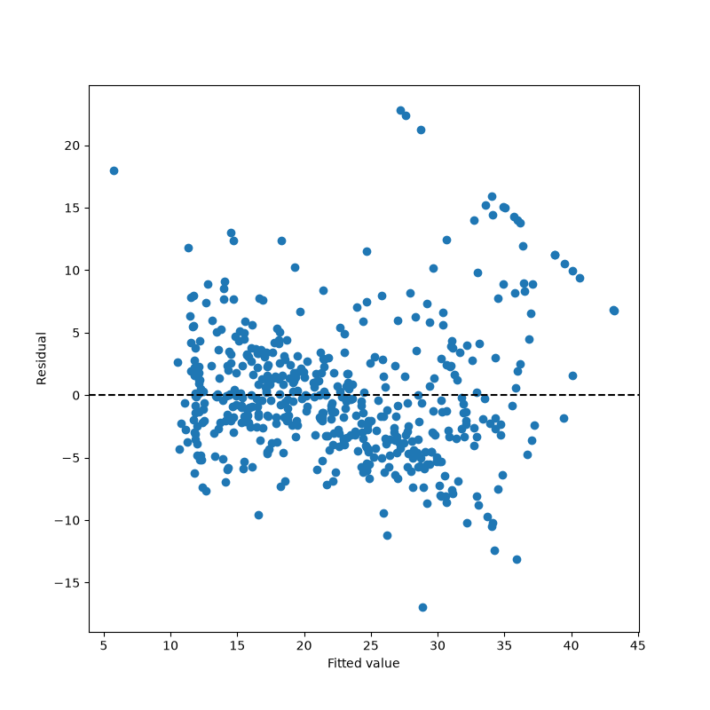
We see that when the quadratic term is included in the model, there is
little discernible pattern in the residuals. In order to create a cubic
or higher-degree polynomial fit, we can simply change the degree
argument to poly().
Qualitative Predictors
Here we use the Carseats data, which is included in the ISLP
package. We will attempt to predict Sales (child car seat sales) in
400 locations based on a number of predictors.
Carseats = load_data('Carseats')
Carseats.columns
['Sales',
 'CompPrice',
 'Income',
 'Advertising',
 'Population',
 'Price',
 'ShelveLoc',
 'Age',
 'Education',
 'Urban',
 'US']
The Carseats data includes several qualitative predictors such as ShelveLoc, an
indicator of the quality of the shelving location — that is, the space within
a store in which the car seat is displayed. The predictor ShelveLoc takes on
three possible values, Bad, Medium, and Good. Given a qualitative variable such
as ShelveLoc, get_dummies generates one column for each value. These variables
are often referred to as a one-hot encoding of the categorical feature. Their
columns sum to one, so to avoid collinearity with an intercept, the first
column is dropped. Below we see the column ShelveLoc_Bad has been dropped,
since Bad is the first level of ShelveLoc. Similarly for the columns Urban and US.
Below we fit a multiple regression model that includes some interaction terms.
Carseats_pd = Carseats.to_pandas()
y = Carseats_pd["Sales"]
Carseats_full = pd.get_dummies(Carseats_pd, drop_first=True)
allvars = list(Carseats_full.columns.drop("Sales"))
final = allvars + [("Income", "Advertising"), ("Price", "Age")]
X = MS(final).fit_transform(Carseats_full)
model = sm.OLS(y, X)
summarize(model.fit())
                      coef  std err       t  P>|t|
intercept           6.5756    1.009   6.519  0.000
CompPrice           0.0929    0.004  22.567  0.000
Income              0.0109    0.003   4.183  0.000
Advertising         0.0702    0.023   3.107  0.002
Population          0.0002    0.000   0.433  0.665
Price              -0.1008    0.007 -13.549  0.000
Age                -0.0579    0.016  -3.633  0.000
Education          -0.0209    0.020  -1.063  0.288
ShelveLoc_Good      4.8487    0.153  31.724  0.000
ShelveLoc_Medium    1.9533    0.126  15.531  0.000
Urban_Yes           0.1402    0.112   1.247  0.213
US_Yes             -0.1576    0.149  -1.058  0.291
Income:Advertising  0.0008    0.000   2.698  0.007
Price:Age           0.0001    0.000   0.801  0.424
In the first line above, we made allvars a list, so that we could add the
interaction terms. Our model-matrix builder has created a ShelveLoc_Good dummy
variable that takes on a value of 1 if the shelving location is good, and 0
otherwise. It has also created a ShelveLoc_Medium dummy variable that equals 1
if the shelving location is medium, and 0 otherwise. A bad shelving location
corresponds to a zero for each of the two dummy variables. The fact that the
coefficient for ShelveLoc_Good in the regression output is positive indicates
that a good shelving location is associated with high sales (relative to a bad
location). And ShelveLoc_Medium has a smaller positive coefficient, indicating
that a medium shelving location leads to higher sales than a bad shelving
location, but lower sales than a good shelving location.