Recurrent Neural Networks
Many sources of data are sequential in nature. Some examples:
- The sequence of words in a document capture narrative, theme and tone: topic classification, sentiment analysis, language translation.
- Time series of temperature, rainfall, wind speed, air quality, etc: forecasting weather or climate.
- Financial time series, market indices, trading volumes, stock and bond prices, exchange rates.
- Recordings of speech, music, other sounds; transcription of text or music, language translation.
- Handwriting, such as doctor’s notes, handwritten digits: OCR
The input to a Recurrent Neural Network is a sequence, be it a sequence of measurements, words, notes, sounds, images, or whatever. The architecture of the network will take advantage of the sequential nature of the input data.
The output can be a sequence, a number or a category.
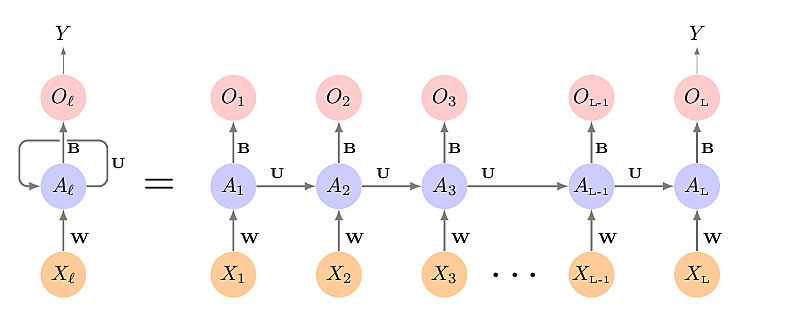
\[ A_{lk} = g \left( w_{k0} + \sum_{j=1}^p w_{kj} X_{lj} + \sum_{s=1}^K u_{ks} A_{l-1,s} \right) \]
where \(g\) is an activation function such as ReLU and
\[ O_l = \beta_0 + \sum_{k=1}^K \beta_k A_{lk} \]
\(W\), \(U\) and \(B\) are the same for each element of the sequence: weight sharing.
For regression problems the loss function is \((Y - O_L)^2\), only referencing the final \(O_L = \beta_0 + \sum_{k=1}^K \beta_k A_{Lk}\) and minimising the sum of squares.
Note that when the desired output \(y\) is a number or category then only \(O_L\) is used; all previous \(O_l\) are discarded, whereas when the desired output is a sequence, all \(\{O_1,\dots, O_L\}\) are used.
Document Classification
Is a movie review positive or negative?
This has to be one of the worst films of the 1990s. When my
friends & I were watching this film (being the target audience it
was aimed at) we just sat & watched the first half an hour with
our jaws touching the floor at how bad it really was. The rest
of the time, everyone else in the theater just started talking to
each other, leaving or generally crying into their popcorn ...
Sentiment analysis makes a judgement about a piece of text whether its sentiment is positive or negative. Some applications:
- Social media monitoring
- Brand reputation management
- Customer feedback analysis
- Market research
- Political analysis
- Healthcare and patient feedback
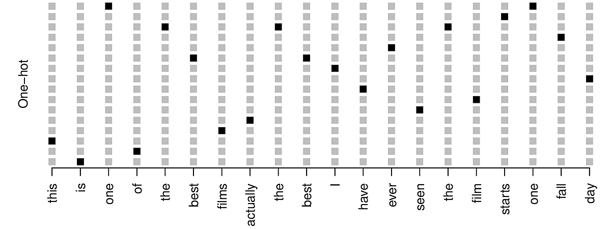
The simplest approach it to treat the text as a bag of words. This takes no account of the order of the words or the structure of the sentences. We can either take the set of words appearing in a text or a bag of words which also counts the number of occurrences of each word.
import heapq
import re
from collections import Counter
from os.path import exists
from sys import exit
from textwrap import wrap

import nltk
import numpy as np
from requests import get

# Download the text of James Joyce's Ulysses from Project Gutenberg
ulysses = "pg4300.txt"
if exists("pg4300.txt"):
    text = open(ulysses).read()
else:
    response = get("https://gutenberg.org/cache/epub/4300/pg4300.txt")
    if response.status_code == 200:
        text = response.text
    else:
        exit("Unable to get text")


def most_popular_words(text, n=100):
    word2count = Counter()
    for sentence in nltk.sent_tokenize(text):
        word2count.update(nltk.word_tokenize(sentence.lower()))

    return heapq.nlargest(n, word2count, key=word2count.get)


for line in wrap(" ".join(most_popular_words(text))):
    print(line)
. , the of and a to in ’ he his i that s : with it _ ? was on you for
) ( her ! him is all at by said as she from or they bloom me not out
be what up my had there like their mr one have but them an t no so
then stephen if when about are which were o your old who this says
down we man over too now do see after did two would time ... off back
will other into eyes know where more those some could hand
But let's consider the set-of-words approach for movie reviews on the IMDb movie database.
One of the most critically acclaimed films of 2023 is Fallen Leaves. Here is one of its reviews on IMDb. It is 147 words long.
text = """A film brimming with charm, thanks to its human characters, struggling in their
own way to make a living. She's a cashier, moving from job to job. She owns her
own apartment. He's a manual laborer who works in a factory, but drinks. And he
goes from job to job. They cross paths. They're both alone. They're drawn to
each other. Girl meets boy. Boy meets girl. They're both shy. But there will be
grains of sand in the mechanics of their relationship. Aki Kaurismäki doses the
construction of this couple perfectly.

Aki Kaurismäki sprinkles his film with references (Jean-Luc Godard, George A.
Romero, for example). The result is a short film, and all the better for it.
There are no unnecessary sequences here. There's no extra-diegetic music.
Without going too fast, Aki Kaurismäki builds the love story between the
characters. A film to warm the heart."""

word_count = len(text.split())
pop_words = most_popular_words(text, 32)
print(word_count)
for line in wrap(" ".join(pop_words)):
    print(line)
147
a the to film job they in s re there of aki kaurismäki with characters
their own she from he but and both girl meets boy for no brimming
charm thanks its
- Kaggle has a dataset of 50k Movie Reviews from IMDb.
- To develop a model, we might limit ourselves to the most popular 10k English words.
- We could make a dataframe of 50k rows and 10k columns, each entry being a
1if the word appears in the review or0if it does not. - Now we have a dataframe with 500 million entries, the vast majority of which
are
0. In fact only about1.3%of the entries are non-zero. Mathematically, such an array is called a sparse matrix and there are methods for dealing with them in Python for Machine Learning such as in SciPy.
from numpy import array
from scipy.sparse import csr_matrix

A = array([[1, 0, 0, 1, 0, 0], [0, 0, 2, 0, 0, 1], [0, 0, 0, 2, 0, 0]])
S = csr_matrix(A)
B = S.todense()

print(A)
print(S)
print(B)
[[1 0 0 1 0 0]
 [0 0 2 0 0 1]
 [0 0 0 2 0 0]]
<Compressed Sparse Row sparse matrix of dtype 'int64'
	with 5 stored elements and shape (3, 6)>
  Coords	Values
  (0, 0)	1
  (0, 3)	1
  (1, 2)	2
  (1, 5)	1
  (2, 3)	2
[[1 0 0 1 0 0]
 [0 0 2 0 0 1]
 [0 0 0 2 0 0]]
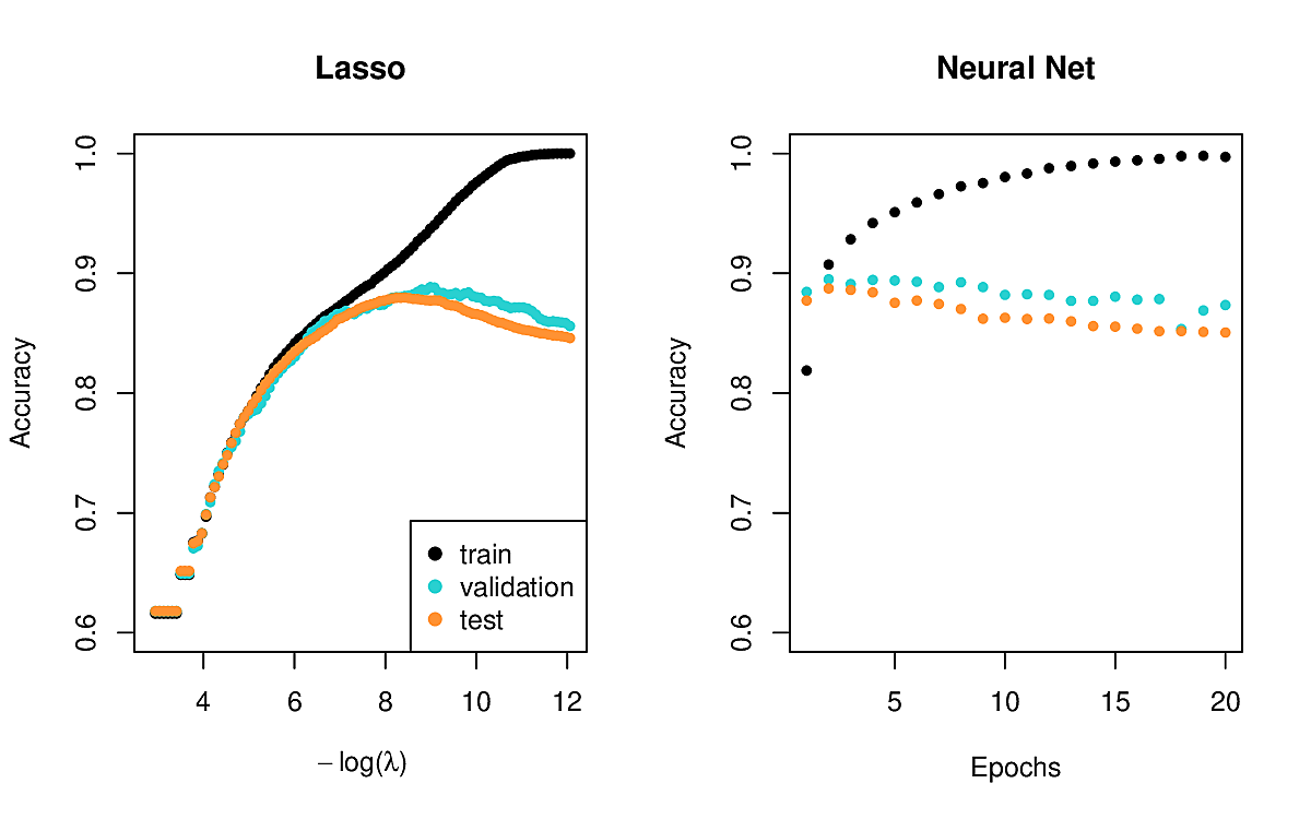
In the Lab you will see an example of taking 25000 reviews and the 10000 most popular words. These are trained on two models.
- A lasso logistic regression
- A neural network with 2 hidden layers, each with 16 ReLU units.
The outcomes are similar.
Note that the bag-of-words approach takes no account of context. For example, the word "blissfully" in the sentence "The movie was blissfully short" might be considered to have a negative sentiment, while in the sentence "The movie was blissfully long", it might be positive. One way to take context into account is to consider a bag of n-grams
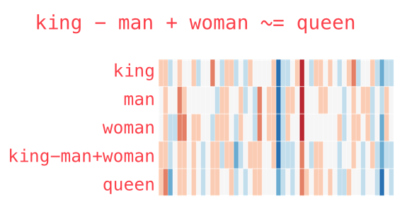
Another approach is to apply dimensionality reduction techniques to reduce the dimension from 10000 in this case to several hundred. This diagram shows 20 words in 16 dimensions.
Here are the words reduced to 5 dimensions.

We call such reductions word embeddings. They have interesting properties.


We can even download some embeddings which pre-trained on large corpora of text using PCA.
We use these embeddings to transform our sparse representations in a large number of dimensions into denser representations in a (much) smaller number of dimensions and feed the results into a RNN.
In the Lab we will train a RNN on a word embedding in 32 dimensions of 25000 IMDb reviews using dropout regularization. This gives an accuracy of around 76%. This can be improved by techniques such as Long short-term memory where two (or more) hidden-layer activations are maintained in order to ensure that early signals are not dominated by later ones. This can improve accuracy to 87%.
Time Series Forecasting
Some historical trading statistics for the New York Stock Exchange from 1962 to 1986. There are 6051 triples.
- Log trading volume
- Dow Jones Index return
- Log volatility
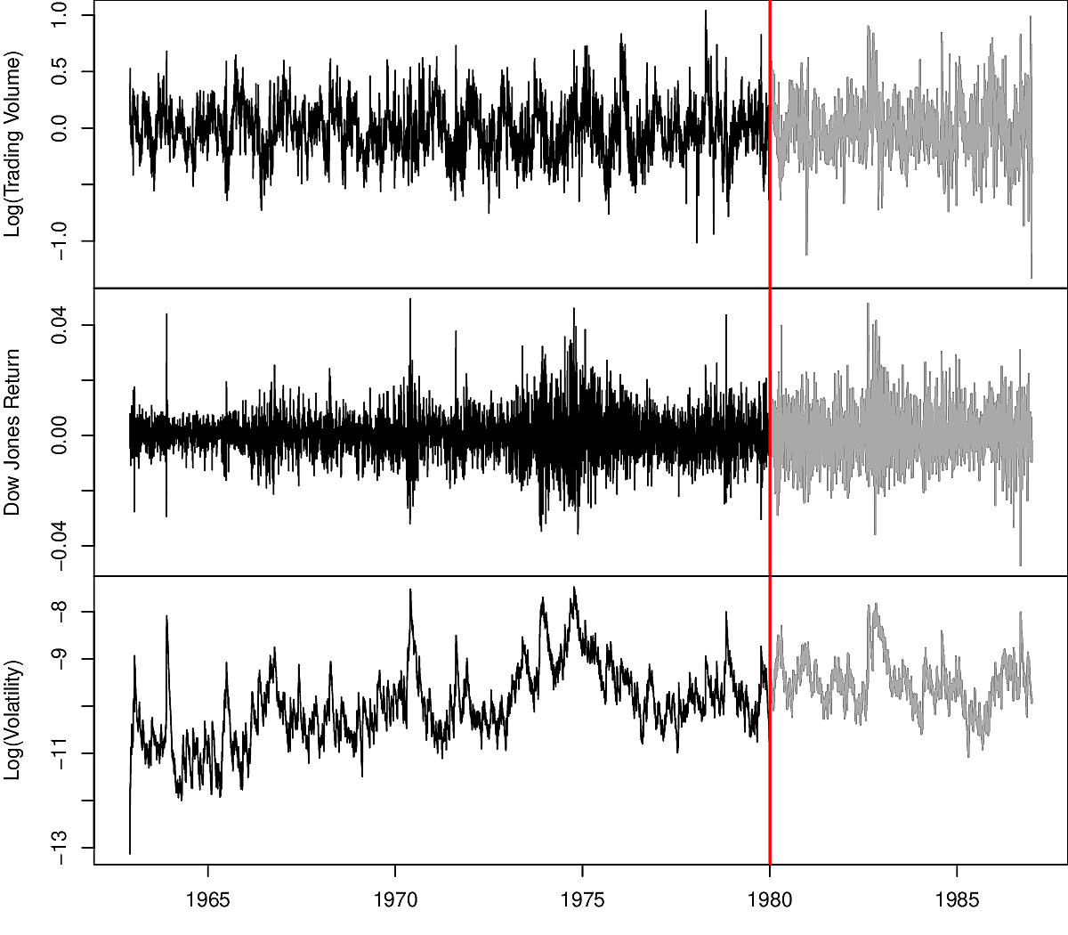
Predicting stock prices is notoriously hard. Predicting volume is easier and can be an indicator of price development.
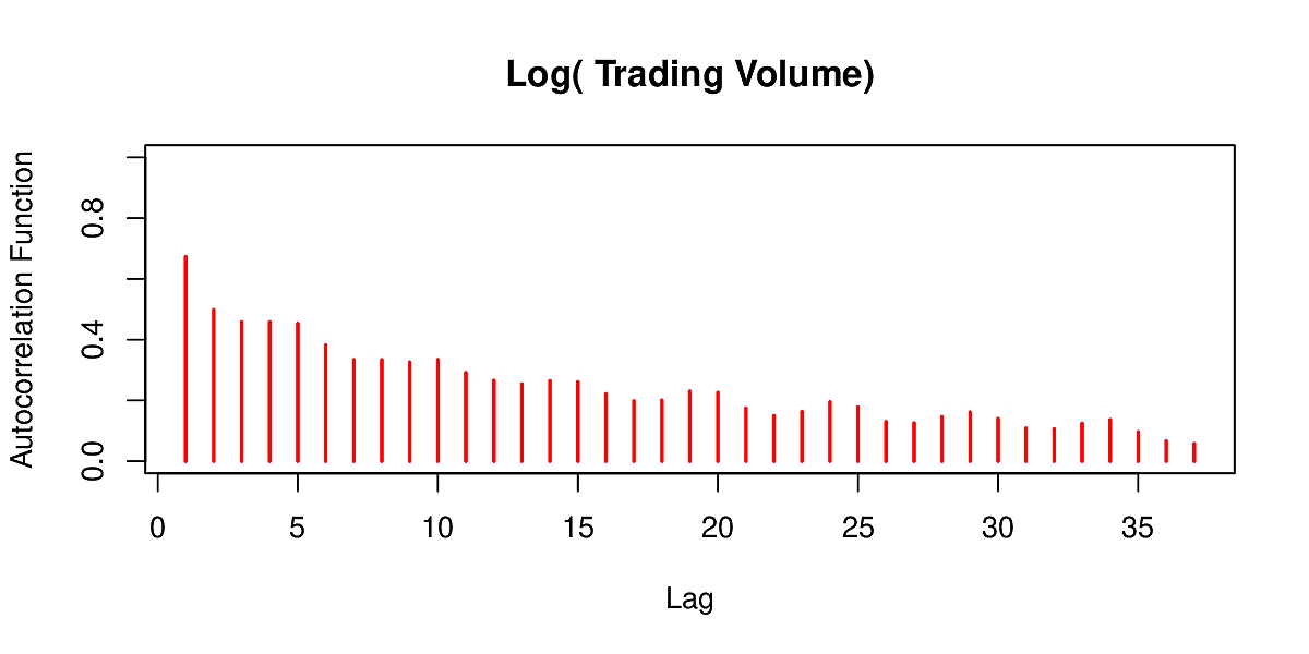
We observe repeating patterns in the series: autocorrelation
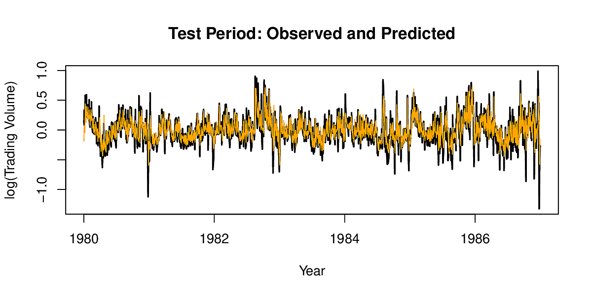
We set out to predict volume from past values of volatility, Dow Jones index and volume. Note that whereas we had 2500 distinct series of data for the IMDb case, here we have 6501 overlapping series. If we use a lag of 5, then we have 6046 pairs in our dataset. Fitting such a RNN we get the following results.
Fitting Neural Networks
If our NN has \(K\) layers, weights \(w_k = (w_{k0}, \dots, w_{kp})\) where \(w_{ij}\) is the weight of unit \(j\) in layer \(i\) , and parameters \(\beta = (\beta_0, \dots, \beta_K)\) and we train it on observations \((x_i, y_i), \; i = 1, \dots, n\), then we seek to minimise
\[ \min_{\{w_k\}_{k=1}^K} \frac{1}{2} \sum_{i=1}^n (y_i - f(x_i))^2 \]
where
\[ f(x_i) = \beta_0 \sum_{k=1}^K \beta_k g\left( w_{k0} + \sum_{j=1}^p w_{kj} x_{ij} \right) \]
Since this is non-linear, we have a nonconvex optimization problem in its parameters so there can be multiple solutions. Local techniques are no longer guaranteed to find the optimal one.
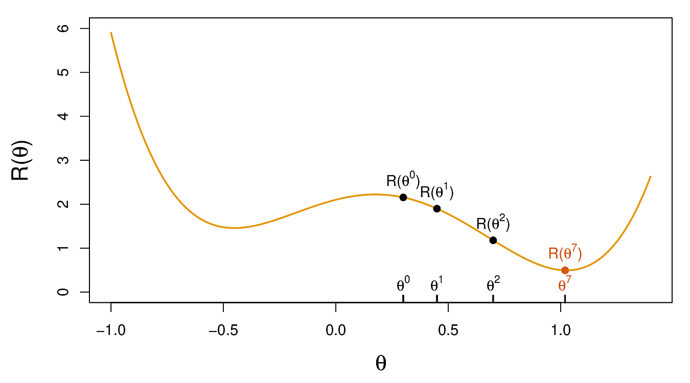
Writing all the parameters in one vector \(\theta\), we seek to minimise the objective \[ R(\theta) = \frac{1}{2} \sum_{i=1}^n (y_i - f_\theta(x_i))^2 \]
Now we do gradient descent as follows
- Guess a value for \(\theta^0\). Set \(t = 0\)
- Now iterate until \(R\) fails to decrease.
- Find a small vector \(\delta\) such that \(R(\theta^{t+1}) = R(\theta^t + \delta) < R(\theta^t)\)
- Set \(t \leftarrow t + 1\)
But how do we find \(\delta\)? We calculate the gradient of \(R\) at \(\theta^t\) \[ \nabla R(\theta^t) = \left. \frac {\partial R(\theta)} {\partial \theta} \right|_{\theta = \theta^t} \]
The gradient points in the direction of greatest increase, i.e. up the slope. We want to go down the direction of greatest decrease so we update \[ \theta^{t+1} \leftarrow \theta^t - \rho \nabla R(\theta^t) \] where \(\rho\) is the learning rate.
The calculation of \(\nabla R\) turns out to be more straightforward than it might seem since we can apply the chain rule for differentiation.
To simplify the presentation, in the following we write \(z_{ik}\) for \(w_{k0} + \sum_{j=1}^p w_{kj} x_{ij}\).
In the case of the \(\beta_k\),
\begin{eqnarray*} \frac{\partial R_i(\theta)}{\partial \beta_k} &=& \frac{\partial R_i(\theta)}{\partial f_\theta(x_i)} . \frac{\partial f_\theta(x_i)}{\partial \beta_k} \\ &=& -(y_i - f_\theta(x_i)) . g(z_{ik}) \end{eqnarray*}And for the \(w_{kj}\),
\begin{eqnarray*} \frac{\partial R_i(\theta)}{\partial w_{kj}} &=& \frac{\partial R_i(\theta)}{\partial f_\theta(x_i)} . \frac{\partial f_\theta(x_i)}{\partial g(z_{ik})} . \frac {\partial g(z_{ik})} {\partial z_{ik}} . \frac {\partial z_{ik}} {\partial w_{kj}}\\ &=& -(y_i - f_\theta(x_i)) \;.\; \beta_k \;.\; g'(z_{ik}) \;.\; x_{ij} \end{eqnarray*}Note that each of these terms is just the residual \(y_i - f_\theta(x_i)\) scaled by a factor and that these fractions of the residual are propagated back through the network in a process called backpropagation.
Examples of RNNs
Google Translate as an example of seq2seq learning
2013: Atari games on YouTube
Considerations: Neural Networks
- Understanding versus prediction
- Understandability
- Explainability
- Occam's Razor
etc
- Advent of Code 2025
- Course Evaluation