Neural Networks & Deep Learning
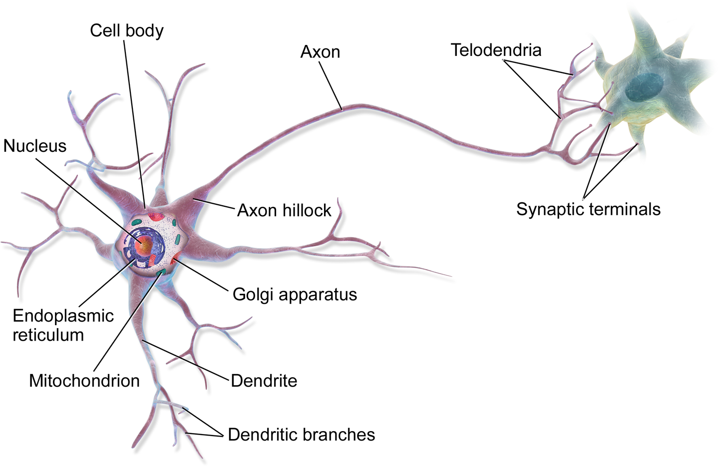
Figure 1: A Biological Neuron
Early history of Artificial Neural Networks
- It is estimated that the average adult human brain contains around 86 billion neurons.
- An axon can be more than 1 metre long.
- Sufficient neurotransmitters in a few milliseconds: fire. Or inhibit.
- Emergent behaviour
- Warren McCulloch & Walter Pitts (1943). Animal brains, propositional logic
- Russel & Whitehead - Principia Mathematica
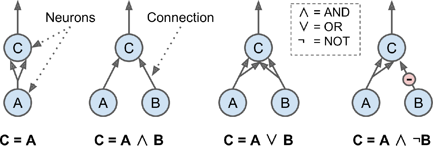
Figure 2: ANNs for propositional logic
Perceptrons
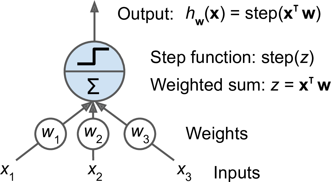
Figure 3: Threshold Logic Unit
- Rosenblatt (1957)
- Weighted sum followed by step function
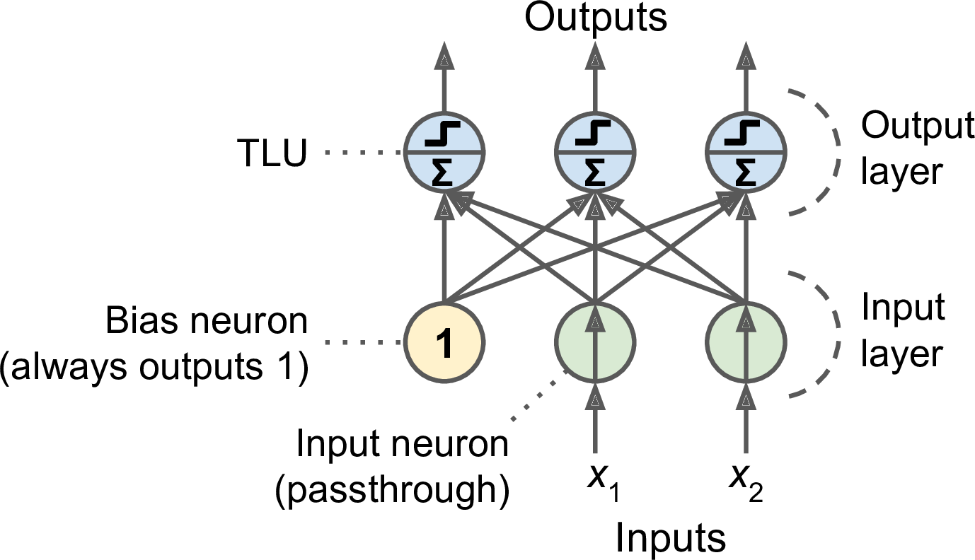
Figure 4: Perceptron
- Linear decision boundary, like Logistic Regression or SVM
- Input layer
- Fully connected layer or dense layer
- Activation function
- Hebb's rule: cells that fire together, wire together
Scikit-Learn Perceptron is SGD. Actually
SGDClassifier(loss="perceptron", learning_rate="constant", eta0=1)
import numpy as np
from sklearn.datasets import load_iris
from sklearn.linear_model import Perceptron

iris = load_iris()

# Take petal length, petal width
X = iris.data[:, (2, 3)]
y = (iris.target == 0).astype(int)

per_clf = Perceptron(max_iter=1000, tol=1e-3)
per_clf.fit(X, y)

per_clf.predict([[2, 0.5]])
- Minsky & Papert (1969). XOR
- AI moves to search, logic, symbolic approaches
Multilayer Perceptrons
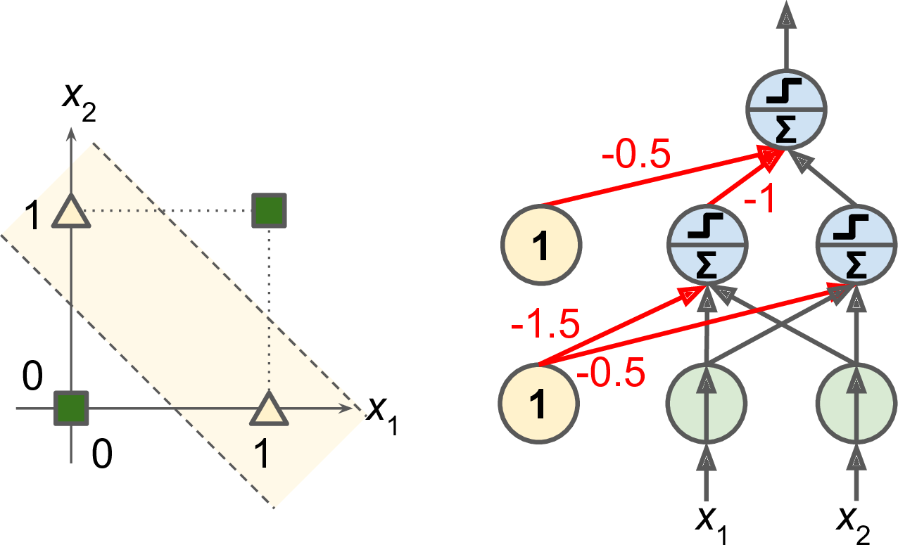
Figure 5: Multilayer Perceptron for XOR
- A Multilayer Perceptron can solve XOR
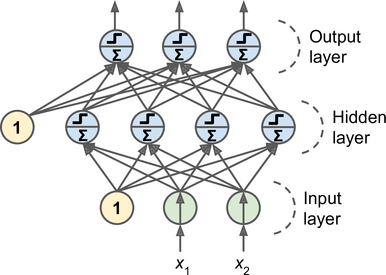
Figure 6: Multilayer Perceptron
- Input, hidden & output layers
- Feedforward
- Network with many layers is deep
- Efficient technique for gradient descent
- Forward pass, backward pass
- Replace step function by sigmoid function so there's always a gradient to work with. \[ \sigma(z) = \frac{1} {1 + e^{-z}} \]
- Need nonlinearity between layers!
- Algorithm. Initialize weights randomly. For each mini-batch or epoch:
- Forward pass. Predict
- Compute output error
- Compute output layer contributions to error by the Chain Rule
- Compute hidden layer contributionsto error, layer by layer, by the Chain Rule
- Compute input layer contributions to error by the Chain Rule
- Update all connection weights by Gradient Descent
- Other activation functions
- Hyperbolic tangent
- on \((-1, 1)\) instead of \((0, 1)\) \[ tanh(z) = 2 \sigma(2z) -1 \]
- Rectified Linear Unit
- not differentiable at 0 and is flat for negative \(z\) but works well in practice (perhaps because it has no asymptote) and has become the default. \[ ReLU(z) = \max(0, z) \]
- Softplus
- smoothed variant of ReLU \[ softplus(z) = \log ( 1 + e^z) \]
- Computes gradient of error w.r.t. every weight using Automated Differentiation
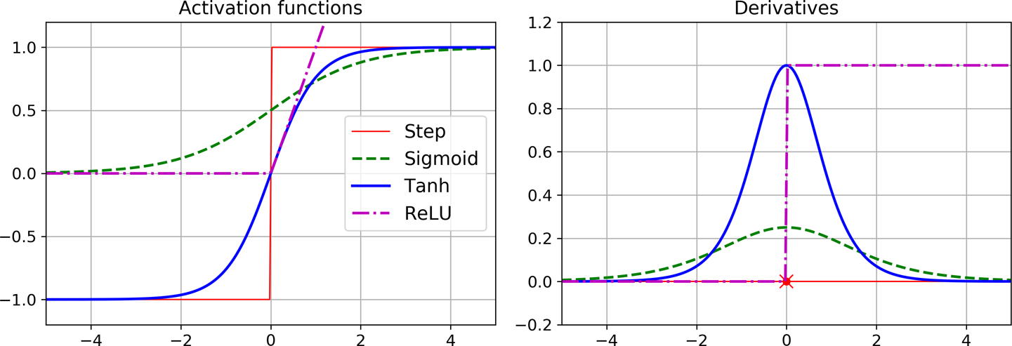
Figure 7: Activation functions
Regression MLPs
- For single value, single output neuron
- For multiple values, one output neuron per dimension
- No activation function on output neurons but transformation to desired range.
- Huber loss function is a combination of MSE and MAE. Converges more quickly and is less sensitive to outliers.
| Hyperparameter | Typical value |
|---|---|
| Input neurons | One per input feature (e.g., 28 x 28 = 784 for MNIST) |
| Hidden layers | 1 to 5 |
| Neurons per hidden layer | 10 to 100 |
| Output neurons | 1 per prediction dimension |
| Hidden activation | ReLU |
| Output activation | None, or transform to range |
| Loss function | MSE or MAE/Huber (if outliers) |
Classification MLPs
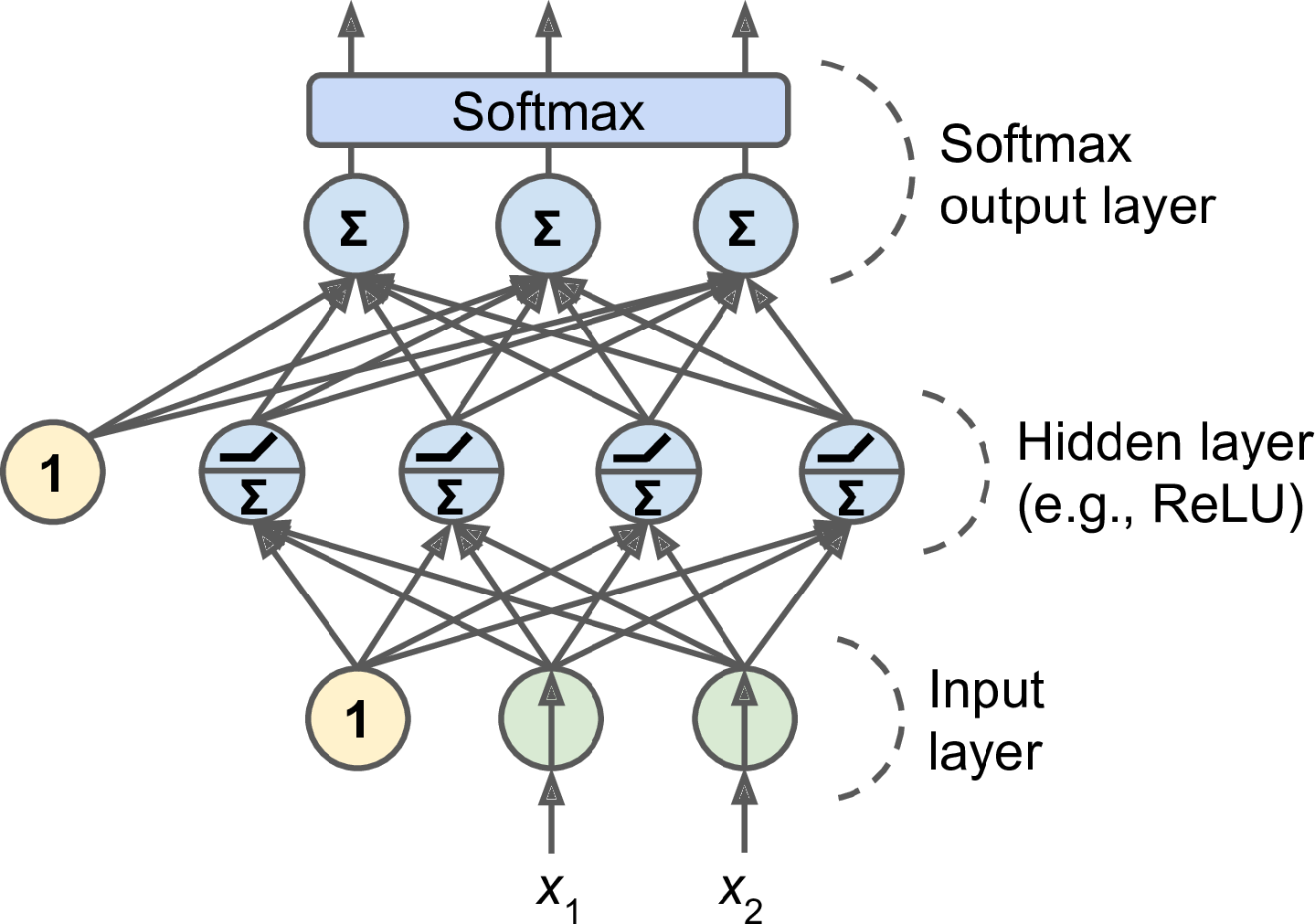
Figure 8: MLP Classifier
- Single, one output neuron per class, or multilabel
- Softmax to ensure output add to one.
- Log loss function (cross-entropy)
Deep Learning
- Why now?
- Huge quantities of data
- Huge increases in compute power. GPUs
- Tweaks in training algorithms
- Funding & progress
- 1965 Multilayer perceptron (Ivakhnenko & Lapa)
- 1967 The Nearest Neighbor Algorithm
- 1967 Stochastic Gradient Descent (Amari)
- 1970 Backpropagation (Linnainmaa)
- 1982 Backpropagation standardised (Werbos)
- 1986 Backpropagation popularised (Rumelhart et al.)
- 1986– Conferences on Neural Information Processing Systems (NIPS)
- 1990 Support Vector Machines (Vapnik) more easily configurable, less tinkering
- 2003 Deep learning for Language models (Bengio et al.)
- 2006 The Facial Recognition Grand Challenge shows significant progress
2013 Atari games
- 2017 Transformer architectures

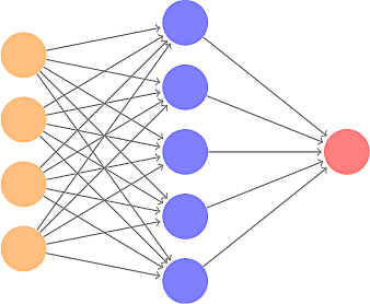
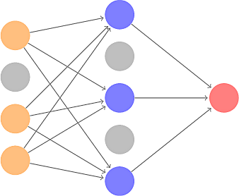
Single Layer Neural Networks
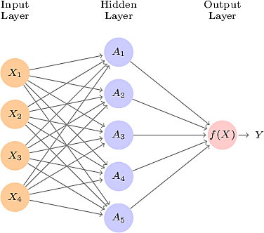
- Feed-forward neural network
- \(p\) input variables \(X = (X_1, \dots, X_p)\), here 4
- One output variable
- Learn a non-linear function \(f(X) = Y\)
- Input layer
- Output layer, here a singleton
- Hidden layer, with \(K\) units, here 5. We call these units the activations
- Each unit in the input layer is connected to each unit in the hidden layer; fully connected
- Each activation \(k\) is calculated from the input layer using its own function \(h_k\) \[ A_k = h_k(X) = g\left( w_{k0} + \sum_{j=1}^p w_{kj} X_j \right) \] The function is a linear combination of the input variables followed by a non-linear function \(g\) which is called the activation function.
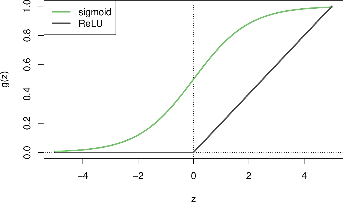
- Early NNs used the sigmoid function \[ \sigma(x) = { 1 \over 1 + e^{-x} } \]
- But the rectified linear unit function or ReLU function is preferred because it is more efficient to store and compute. \[ g(x) = (x)_+ = \begin{cases} 0, & \text{if } x < 0 \\ x, & \text{otherwise} \end{cases} \]
- Our NN computes 5 new features which are linear combinations of the input vector and then non-linearizes them using \(g\). In the absence of the non-linear function \(g\), we would have merely a linear model. It allows us to capture complex nonlinearities and interaction effects.
- The analogy is with a neuron in the brain being fired or inhibited by the activations of its synapses.
- Activations close to \(1\) are firing while those close to \(0\) are silent.
- Now we have
- To fit a NN, requires us to estimate the unknown parameters in this equation, namely \(\beta_0, \dots, \beta_K\) and \(w_{k0}, \dots, w_{kp}\), a total of \(5 + 4 = 9\). These values are collectively known as the weights.
- For a regression problem we use squared-error loss and minimize \[ \sum_{i=1}^n (y_i - f(x_i))^2 \]
- We will look at techniques for minimization later.
Multilayer Neural Networks
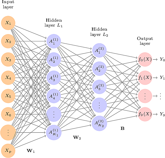
- When we have multiple hidden layers, we speak of a Multilayer Neural Networks
- Between each pair of adjacent layers, except the last pair, the activations of the layer on the right are linear combinations of the layer on the left followed by the application of a non-linear activation function.
- The last layer is a linear combination of the activations of the penultimate layer.
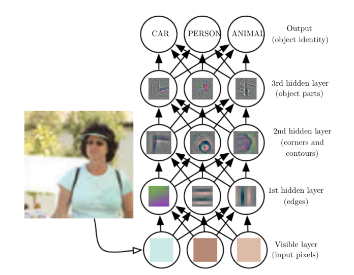
- The first hidden layer computes non-linear features of the input layer.
- The second hidden layer computes non-linear features of the features in the first hidden layer.
The MNIST handwritten digit dataset
The task of recognising handwritten digits drove much research into NNs in the late 1980s. The challenge was that it is a task that is easy for humans since a large part of our brains is dedicated to processing visual information but, at the time, was difficult for computers.
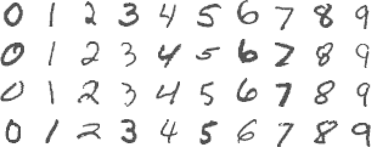
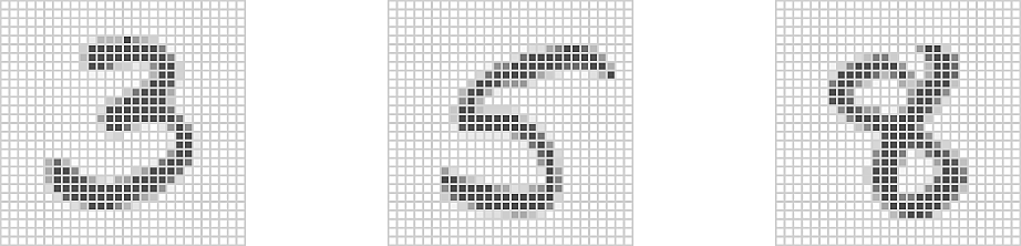
- 60000 training images
- 10000 test images
- Each image has \(p = 28 \times 28 = 784\) pixels
- Each pixel is an 8-bit greyscale value in the range \([0,255)\)
- The output is a one-hot encoded vector \(Y = (Y_0, Y_1, \dots, Y_9)\)
- In the architecture of the network above, we have \(784\) input units, corresponding to each of the pixels.
- We have two hidden layers, one with \(256\) units and one with \(128\) units.
- The output layer has \(10\) units, corresponding to the \(10\) digits. Here we use one-hot encoding but we might wish to predict several responses at once: multi-task learning
- Note that we have a total of \(784 \times 257 + 257 \times 129 + 129 \times 10 = 236188\) weights to minimize over.
- If we were doing multi-task learning we would leave the activations of our output units as they are and set \(Y_m = f_m(X)\) but for classification we would like the output values to be interpretable as probabilities. For this we can use the softmax function which is a normalized exponential function. \[ Y_k= \sigma(f_k(X)) = { e^{f_k(X)} \over \sum_{m=1}^M e^{f_m(X)} } \]
- Now the classifier can assign each image to the class with the highest probability.
- Since our task is classification rather than regression we use an information-theoretic quantity called the cross-entropy. It is a measure of the amount of information needed to identify events drawn from one distribution when the events are encoded using the other distribution. What it comes down to is that the quantity we need to minimize is \[ - \sum_{i=1}^n \sum_{m=0}^9 y_{im} \log(f_m(x_i)) \]
So how does our NN do on the MNIST dataset in comparison to other methods?
Method Test Error Linear Discriminant Analysis 12.7% Multinomial Logistic Regression 7.2% Neural Network + Ridge Regularization 2.3% Neural Network + Dropout Regularization 1.8%
Convolutional Neural Networks
CIFAR100 is a database of small images.
- There are100 classes containing 600 images each.
- There are 60000 images in total, a 50000 image training set and a 10000 test set.
- Each image is 32x32 pixels of 8-bit RGB colour.
- The classes are grouped in 20 superclasses.
- Each image is labelled by class and superclass.
- The criteria for deciding whether an image belongs to a class were as
follows:
- The class name should be high on the list of likely answers to the question “What is in this picture?”
- The image should be photo-realistic. Labelers were instructed to reject line drawings.
- The image should contain only one prominent instance of the object to which the class refers.
- The object may be partially occluded or seen from an unusual viewpoint as long as its identity is still clear to the labeler.
| Superclass | Classes |
|---|---|
| aquatic mammals | beaver, dolphin, otter, seal, whale |
| fish | aquarium fish, flatfish, ray, shark, trout |
| flowers | orchids, poppies, roses, sunflowers, tulips |
| food containers | bottles, bowls, cans, cups, plates |
| fruit and vegetables | apples, mushrooms, oranges, pears, sweet peppers |
| household electrical devices | clock, computer keyboard, lamp, telephone, television |
| household furniture | bed, chair, couch, table, wardrobe |
| insects | bee, beetle, butterfly, caterpillar, cockroach |
| large carnivores | bear, leopard, lion, tiger, wolf |
| large man-made outdoor things | bridge, castle, house, road, skyscraper |
| large natural outdoor scenes | cloud, forest, mountain, plain, sea |
| large omnivores and herbivores | camel, cattle, chimpanzee, elephant, kangaroo |
| medium-sized mammals | fox, porcupine, possum, raccoon, skunk |
| non-insect invertebrates | crab, lobster, snail, spider, worm |
| people | baby, boy, girl, man, woman |
| reptiles | crocodile, dinosaur, lizard, snake, turtle |
| small mammals | hamster, mouse, rabbit, shrew, squirrel |
| trees | maple, oak, palm, pine, willow |
| vehicles 1 | bicycle, bus, motorcycle, pickup truck, train |
| vehicles 2 | lawn-mower, rocket, streetcar, tank, tractor |
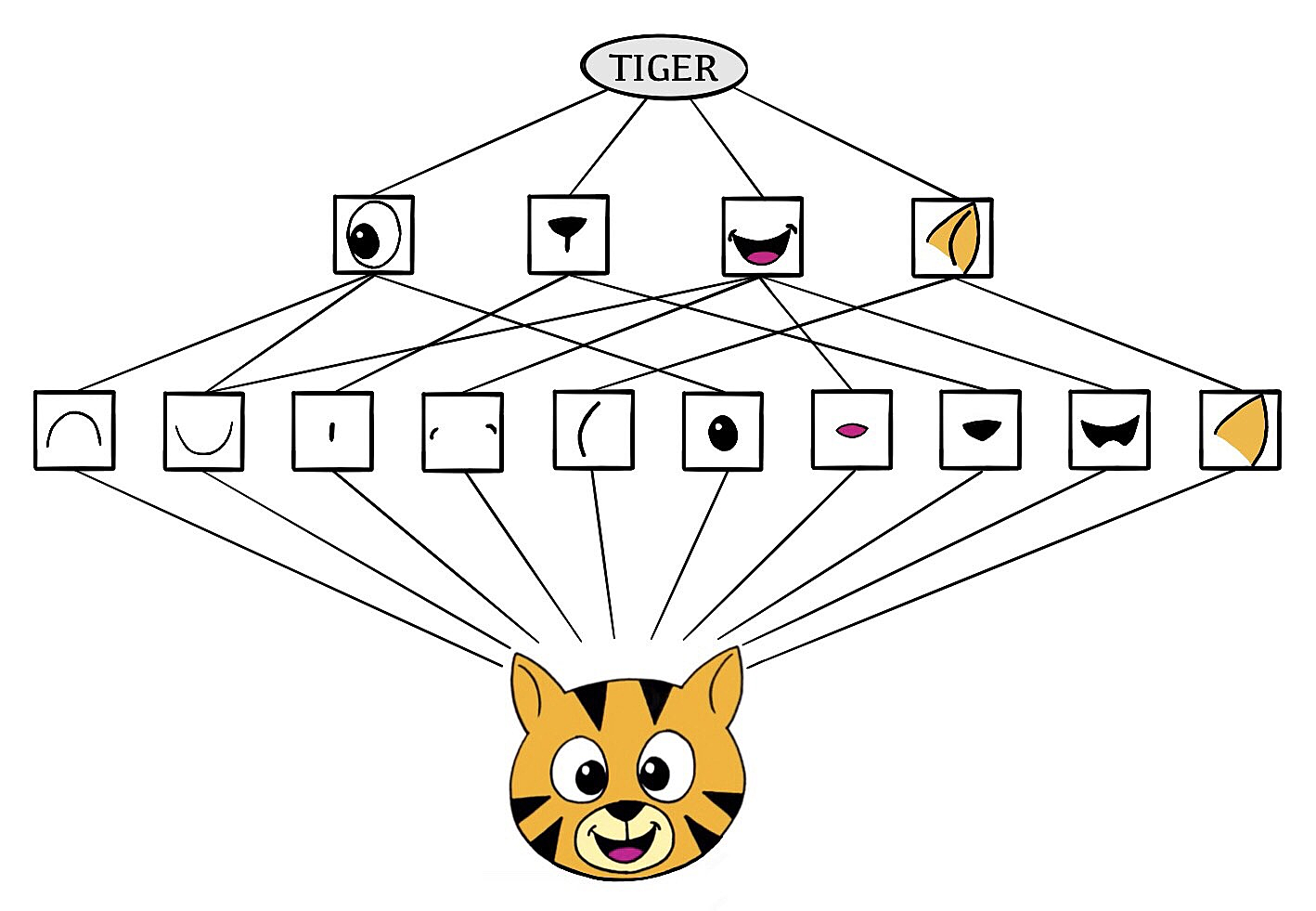
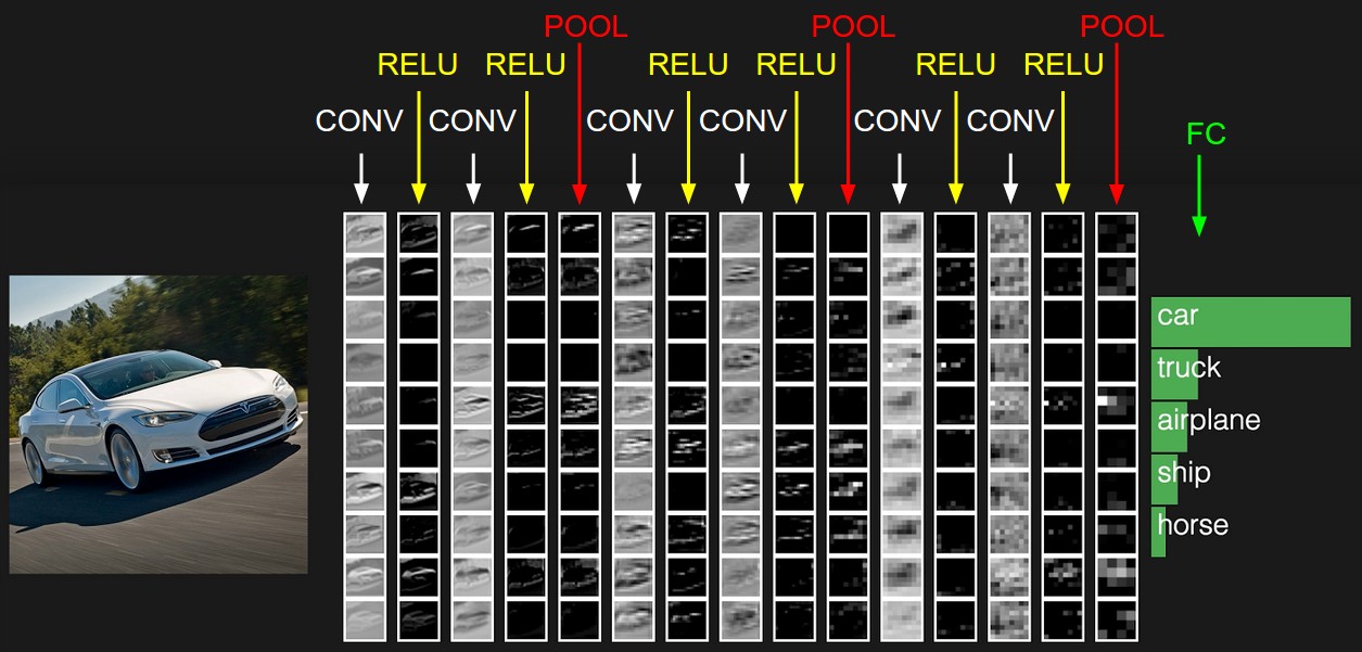
Convolutional Neural Networks (CNN) are intended to mimic human vision by first identifying smaller local features, then compound features, then complete images. They introduce two kinds of layer:
- convolution layers
- search for instances of small pattern in the image.
- pooling layers
- downsample features to select prominent subsets.
Standard sets of convolution filters are used in image processing but CNNs learn the features from training data.
CNNs have proved successful in
- image recognition
- video analysis
- natural language processing
- anomaly detection
- games such as checkers and go


Data augmentation can give us more perspectives of images by distorting them in natural ways. When doing SGD in batches, we can generate a batch by augmenting a single image in various ways.
Pretrained classifier
resnet50 is a CNN image classifier by He et al.
- 50 layers
- Trained on the ImageNet image database of more than 14 million hand-annotated images.
You can download the network pre-trained, freeze the weights of the, add some layers and train them to fine-tune the composite network to your own dataset.
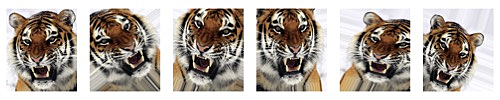
Here is how resnet50 performs on some images from the book authors' personal
collection.
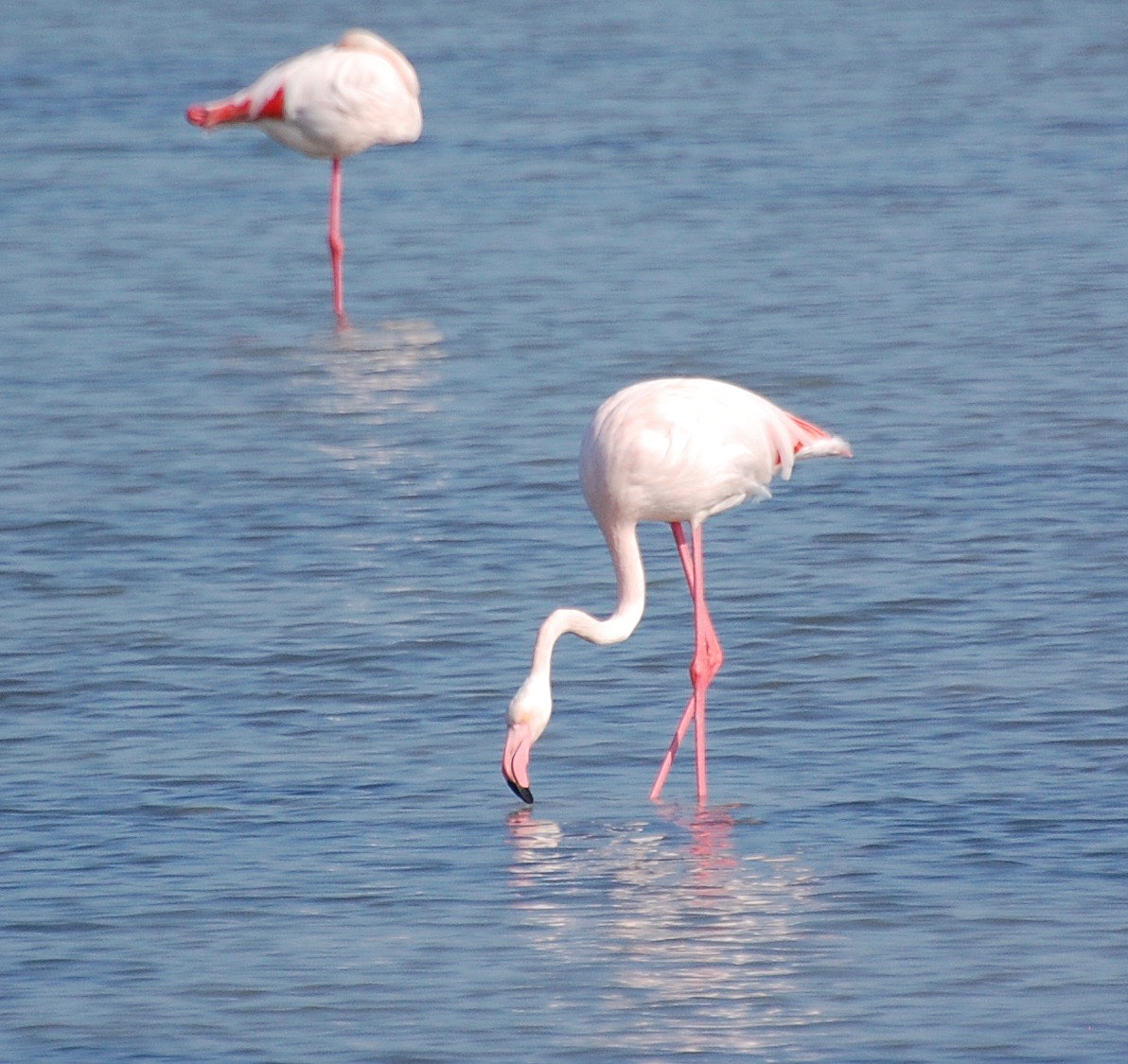
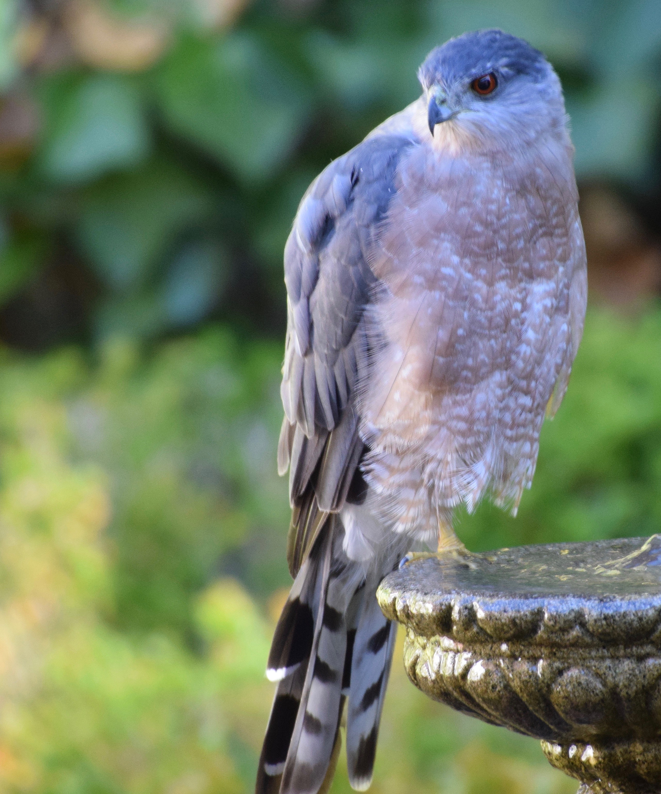
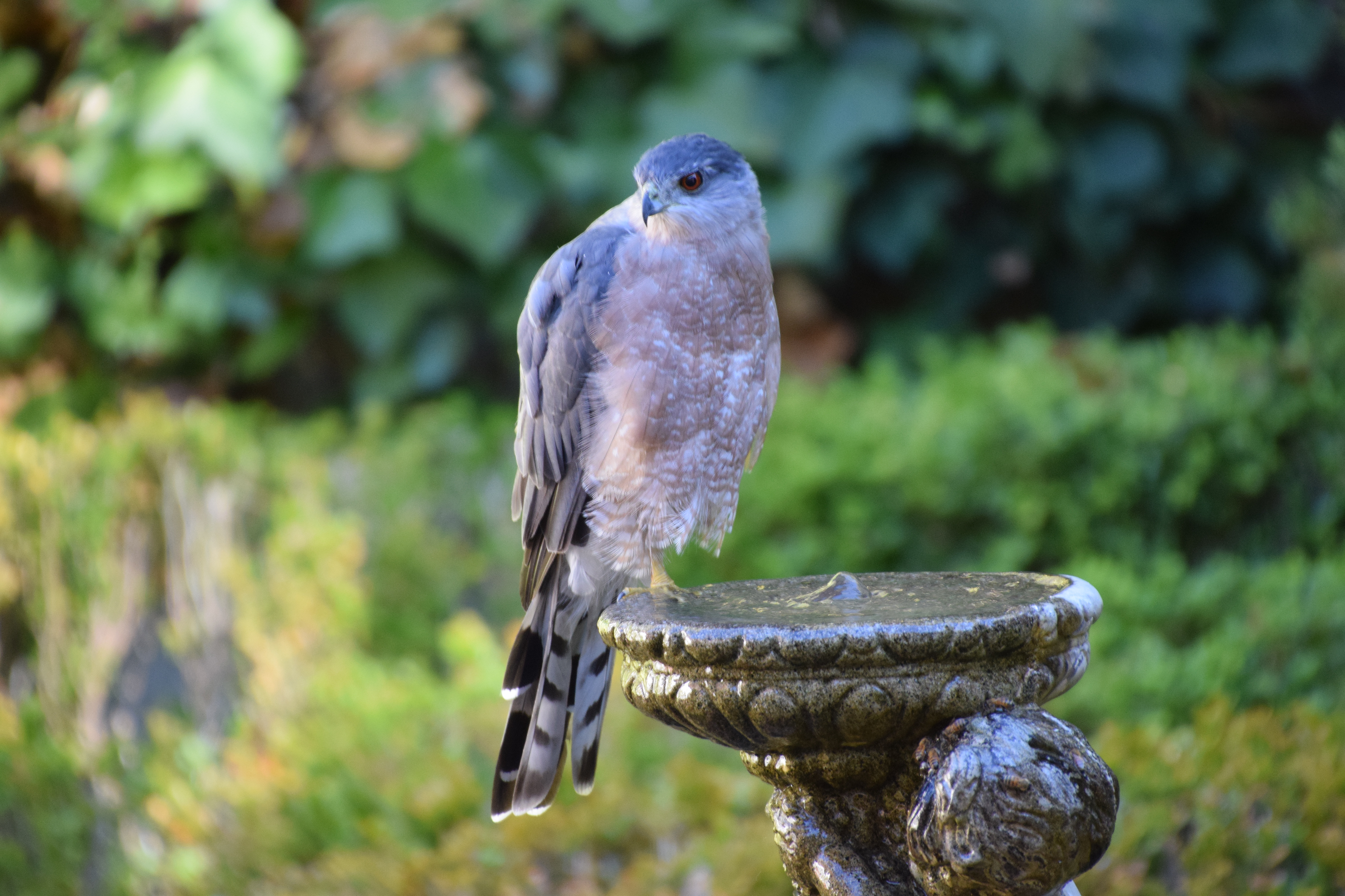
| flamingo | Cooper’s hawk | Cooper’s hawk | |||
|---|---|---|---|---|---|
| flamingo | 0.83 | kite | 0.60 | fountain | 0.35 |
| spoonbill | 0.17 | great grey owl | 0.09 | nail | 0.12 |
| white stork | 0.00 | robin | 0.06 | hook | 0.07 |
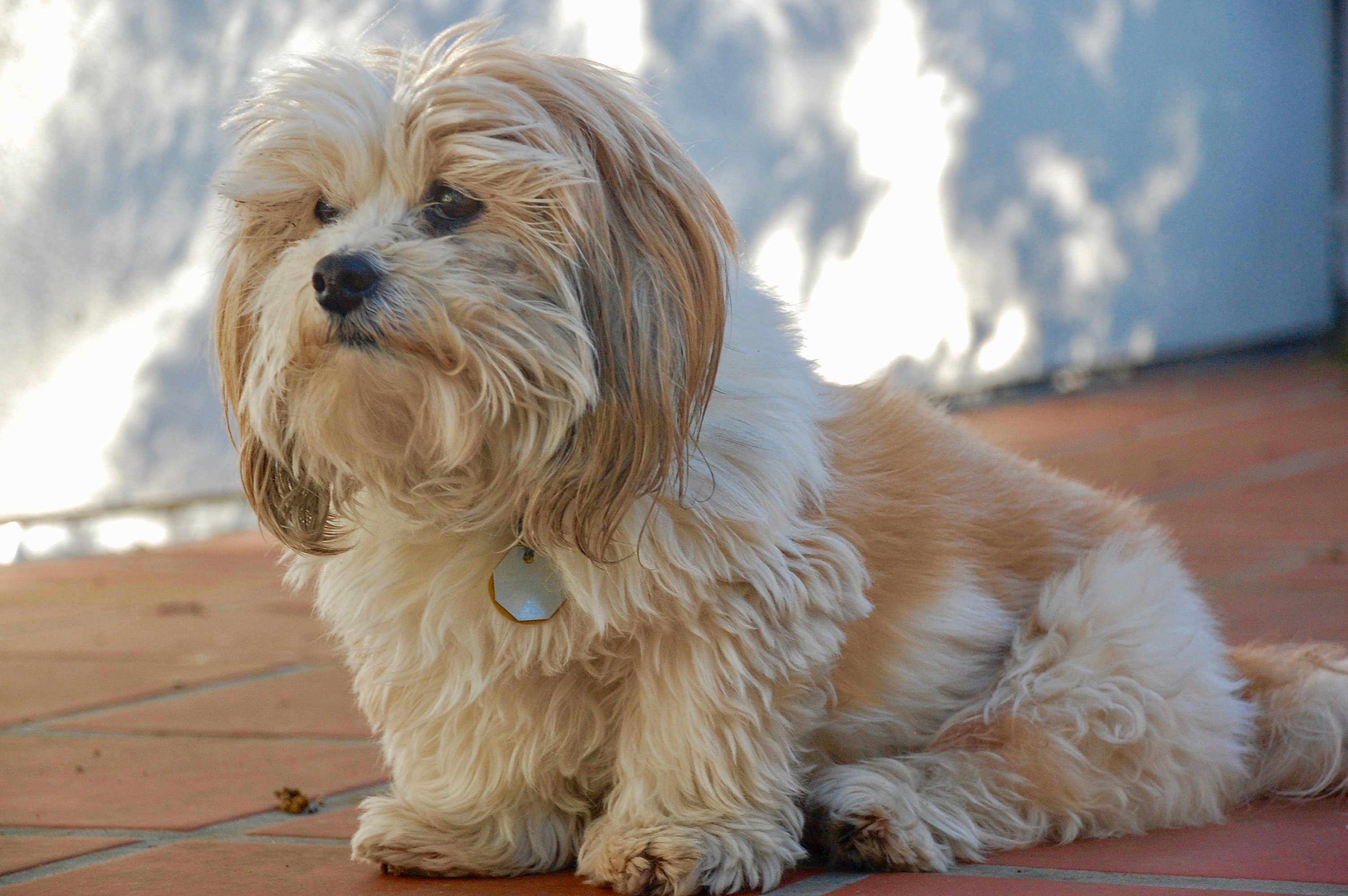
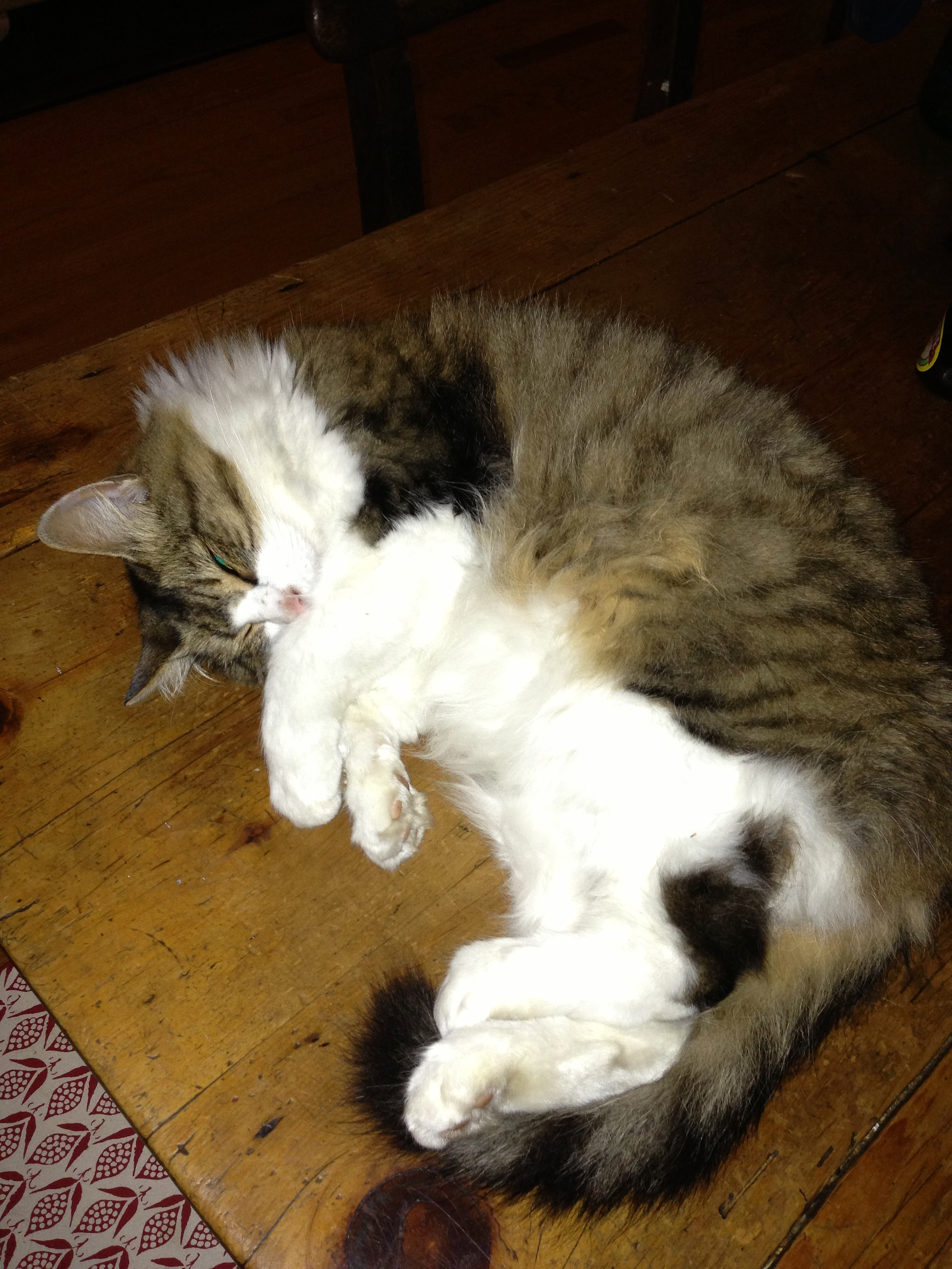
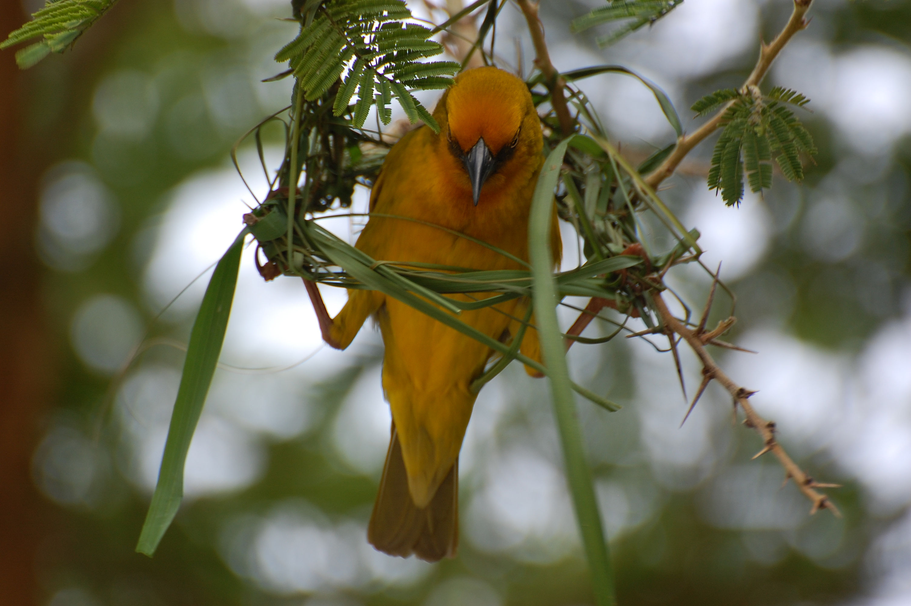
| Lhasa Apso | cat | Cape weaver | |||
|---|---|---|---|---|---|
| Tibetan terrier | 0.56 | Old English sheepdog | 0.82 | jacamar | 0.28 |
| Lhasa | 0.32 | Shih-Tzu | 0.04 | macaw | 0.12 |
| cocker spaniel | 0.03 | Persian cat | 0.04 | robin | 0.12 |
Dropout Learning
Dropout learning is a kind of regularization. For each training image a fraction \(\phi\) of the units are removed by setting their activation to zero. The weights of the remaining units are scaled up by \(1 / (1 - \phi)\) to compensate. Dropout learning has been shown to mitigate overfitting.
Tensorflow Playground
etc
- Emacs config