Imputation, Clustering & Recommender Systems

Two weeks ago we did Principal Component Analysis and its application to

Dimensionality reduction
Visualization
Noise filtering
Facial recognition

Today we go on to look at unsupervised learning for imputation, clustering & recommender systems.

Imputation

Often real-world datasets have missing values. There can be many reasons for this, such as

Data may have been copied carelessly or mislabelled.
Data files may have been corrupted.
Sensors may have failed.
Human error.

How can we deal with missing values? Depending on the underlying cause of the missing data, we may want to treat our dataset in different ways.

Imagine a hospital where every patient should be weighed upon admission. In the resulting dataset it turns out that some patient weights are missing. Consider three scenarios for the missing data.

The weighing scales was faulty and sometimes didn't give a reading.
The nurse who worked admissions on Tuesdays and Thursdays wasn't aware that patients should be weighted.
Some patients are so obese that the admission nurses didn't dare to put them on the scales.

The data in Scenario 1 seem to be missing at random while there is some pattern in the missing values for Scenario 2. However in Scenario 3 the missing data tell a story and provide a signal that could be potentially important for the patient's treatment.

Sometimes data are missing by design. For example suppose Netflix has an $n \times p$ dataframe holding the ratings given by $n$ clients for $p$ movies where $p$ is in the order of thousands. It is unlikely that any client will have seen a fraction of all of the movies so many of the entries will be empty.

We call the process of finding suitable values for the missing values imputation.

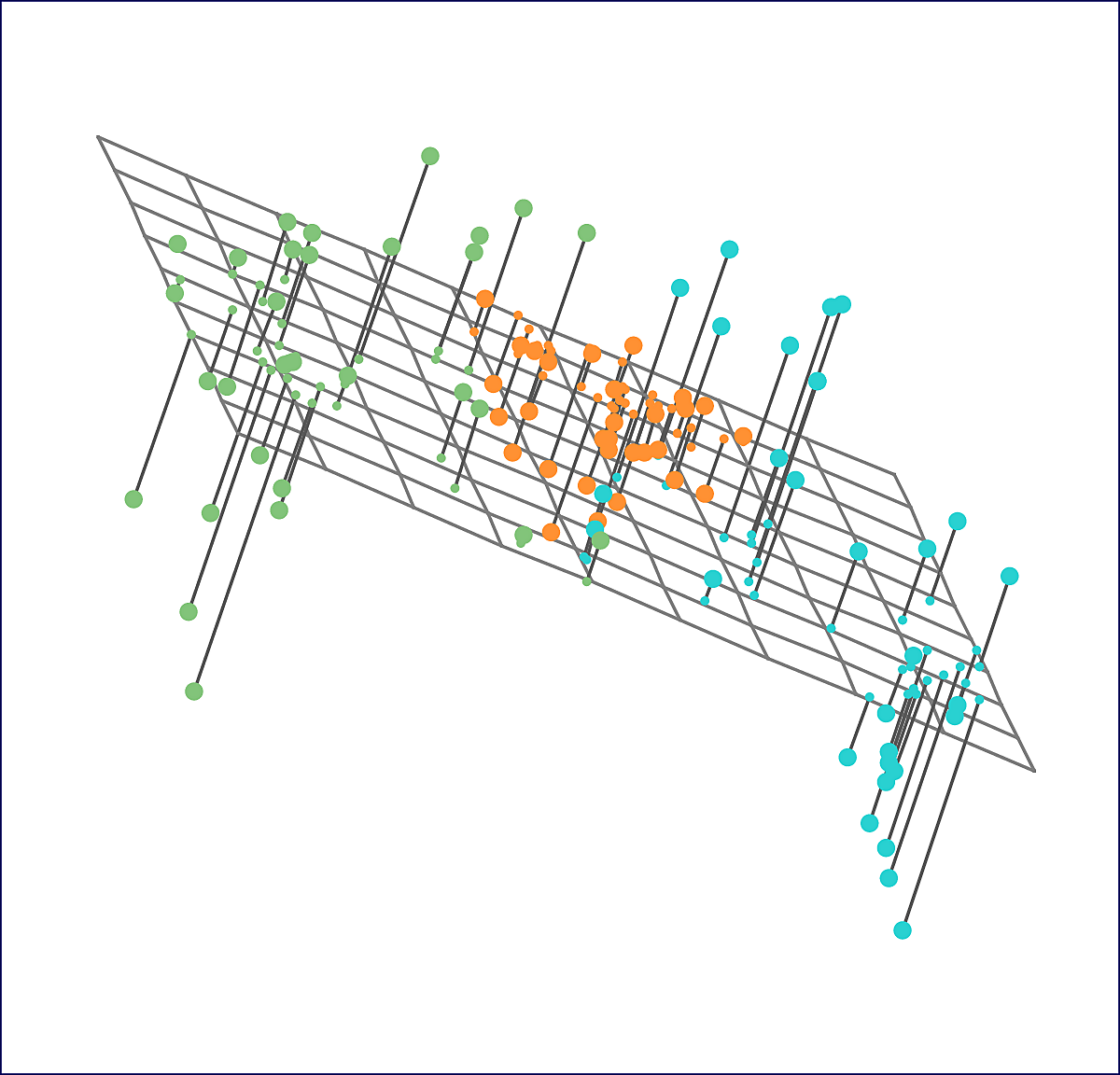
We can formally state the problem of finding principal components as follows. The best $M$-dimensional approximation for the $j$-th component of the $i$-th observation $x_{ij}$ is

\[ x_{ij} \approx \sum_{m=1}^M z_{im} \phi_{jm} \]

So we are looking for the best $\hat{x}_{ij} \approx \sum_{m=1}^M a_{im} b_{jm}$ for which

\[ \min_{A \in \mathbb{R}^{m \times N}, B \in \mathbb{R}^{p \times N}} \Biggl\{ \sum_{j=1}^p \sum_{i=1}^n \left( x_{ij} - \sum_{m=1}^M a_{im} b_{jm} \right)^2 \Biggr\} \]

The matrices $A$ and $B$ which minimize the above give us the best approximation for the weights $z_{im}$ and loading vectors $\phi_{jm}$.

It turns out that a variant of the PCA algorithm can be used to find the principal components and impute missing values at the same time using the modified optimization problem.

\[ \min_{A \in \mathbb{R}^{m \times N}, B \in \mathbb{R}^{p \times N}} \Biggl\{ \sum_{(i,j) \in \mathcal{O}} \left( x_{ij} - \sum_{m=1}^M a_{im} b_{jm} \right)^2 \Biggr\} \]

We run this on the USArrests data set (with 4 columns and 50 rows) where we synthetically remove 10% of the values as follows.

Standardize each variable to mean zero and standard deviation one.
Randomly select 20 of the 50 states.
For each such state, randomly set one of the four values to zero.

We apply the hard-impute iterative algorithm for matrix completion using only a single principal component. We repeat 100 times and find that the correlation between the imputed values and the removed values is 0.63 with a standard deviation of 0.11

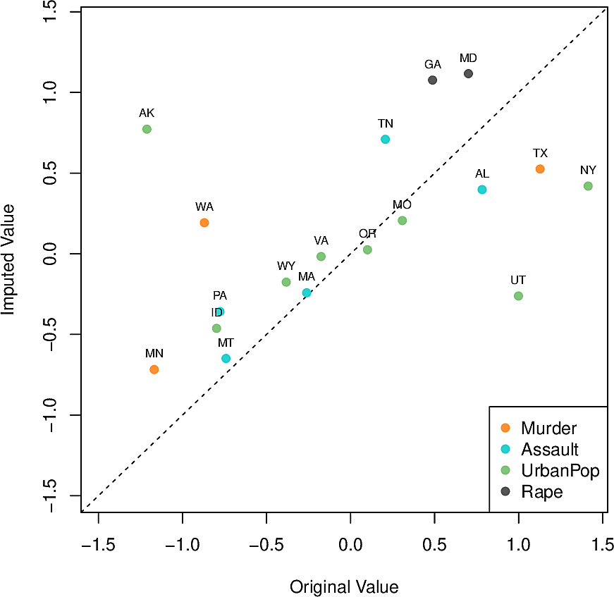
If we had done it with the complete dataset, the correlation on the (unattainable) first principal component would have been 0.79 so this is pretty good.

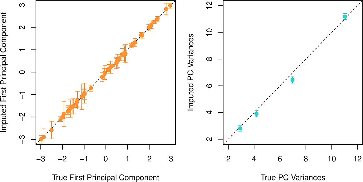
The method can be applied taking more principal components, the number being determined by a method similar to the validation-set approach where we remove and restore values.

Recommender Systems

Companies such as Netflix, Amazon and Bol use data about customer preferences in the past to recommend purchases for the future.

In 2006 Netflix famously released a dataset consisting of the preferences of 480,189 customers for 17,770 moves with the challenge to find the best prediction model. On average the customers had seen about 200 movies meaning that about 99% of the values were missing. The prize of $1,000,000 was won by BellKor's Pragmatic Chaos team.

Jerry Maguire				3	5	3			3
Oceans			2		1
Road to Perdition		3					5
A Fortunate Man			4
Catch Me If You Can	4				4				5
Driving Miss Daisy							2
The Two Popes		3			4
The Laundromat								3	1
Code 8			2
The Social Network		3

The thinking behind the approach is that many customers will have overlapping movies with other customers. Among those overlapping movies will be movies for which the customers have similar preferences.

Again writing $\hat{x}_{ij} \approx \sum_{m=1}^M \hat{a}_{im} \hat{b}_{jm}$ , we can interpret the components as

cliques: $\hat{a}_{im}$ is the strength by which the $i$-th customer belongs to the $m$-th clique.
genres: $\hat{b}_{jm}$ is the strength with which the $j$-th movie belongs to the $m$-th genre.

Examples of genres are westerns, romcoms , fantasy or action movies.

Clustering Methods

Clustering refers to a large number of methods designed to partition data points into groups which we call clusters. The idea is that two data points from distinct clusters should somehow be more different that two data points from the same cluster. Of course we need to define what we mean by different.

Scikit-learn offers many clustering methods each of which might be more or less suitable for various kinds of dataset.

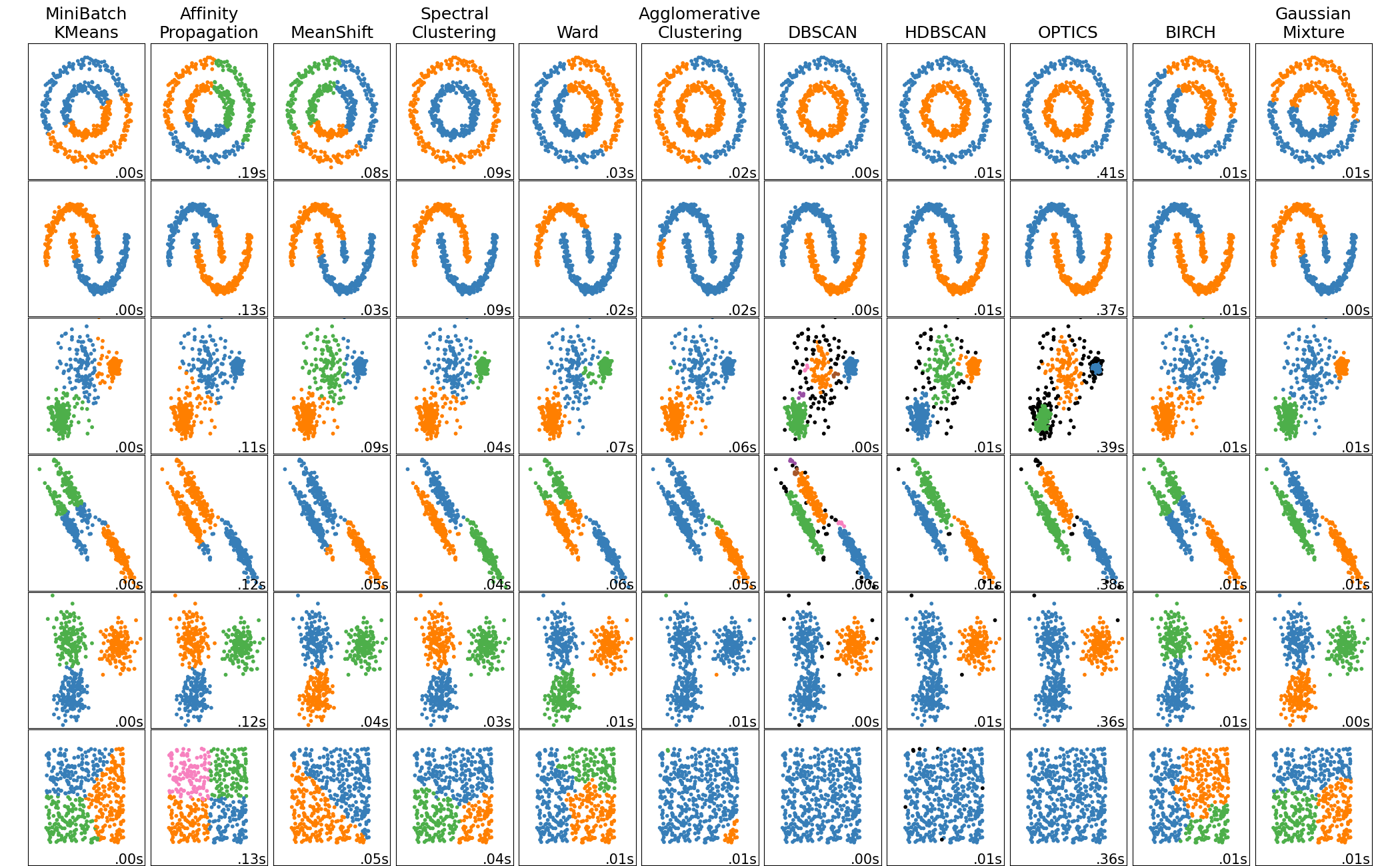
Clustering is used in data exploration to look for structure in the data and to understand it better. Where PCA looks to find a low-dimensional representation of the data, clustering seeks homogeneous subgroups.

Examples of clustering:

We have a number of observations for patients with a medical condition and we suspect that there may be more than one underlying cause.
We have a number of observations about the behaviour of consumers and we would like to identify subgroups to whom we could market products in a targeted way. This is known as market segmentation.

K-means clustering

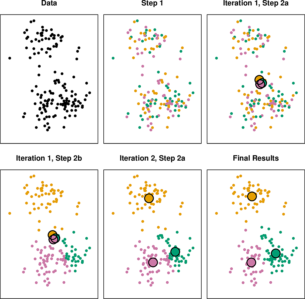
We set out to divide our dataset into $K$ clusters. The idea for the algorithm is simple.

First we assign the data points randomly to the $K$ clusters.
Now we iterate until the clusters stabilize.
1. We compute the centroid of each cluster.
2. We assign each data point to the cluster with centroid nearest to it.

At some point the clusters stabilize in the sense that no point moves from cluster to cluster during an iteration.

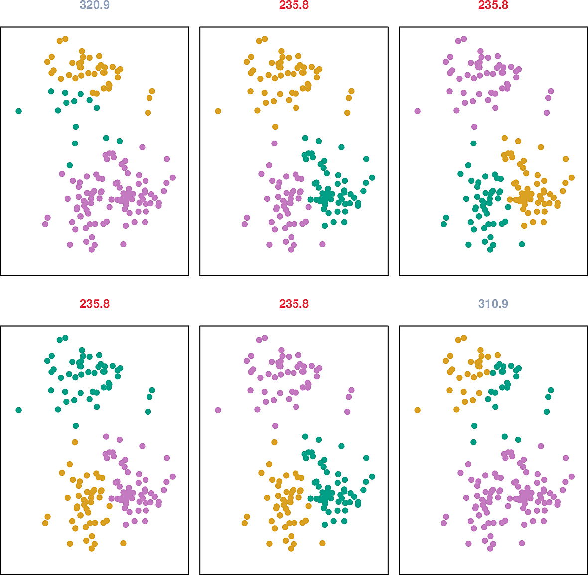
The process works pretty well in practice but it stabilizes at a local optimum which is not guaranteed to be global. Approaches to dealing with this are to ensure that the initial allocation is well distributed and to repeat the process several times and choose one with the lowest objective.

Let $C_i, i=1\dots K$ be a partition of the observations. Let $W(C_i)$ be the within-cluster variation of cluster $i$. The within-cluster variation could, for example, be defined as the sum of the Euclidean distances between each pair of points in the cluster. For a given $K$ we need to minimize the objective:

\[ \min_{C_1, \dots, C_K} \sum_{k=1}^K W(C_k) \]

Here are some example runs, together with the value of the objective at stabilization.

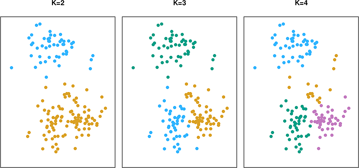
The problem of selecting the best value of $K$ can be subjective. We will examine it more closely in the next section.

Hierarchical clustering

Instead of having to specify in advance how many clusters we want, we could take an approach of having sub-clusters and sub-sub-clusters and so on. We call this hierarchical clustering.

Two approaches are possible. We could start with the entire dataset, split it and iterate. This is the top-down approach.

Or we could start with the individual data points and join them into clusters which we then iteratively join. This is the bottom-up or agglomerative approach. It leads to rather pretty diagrams called dendrograms

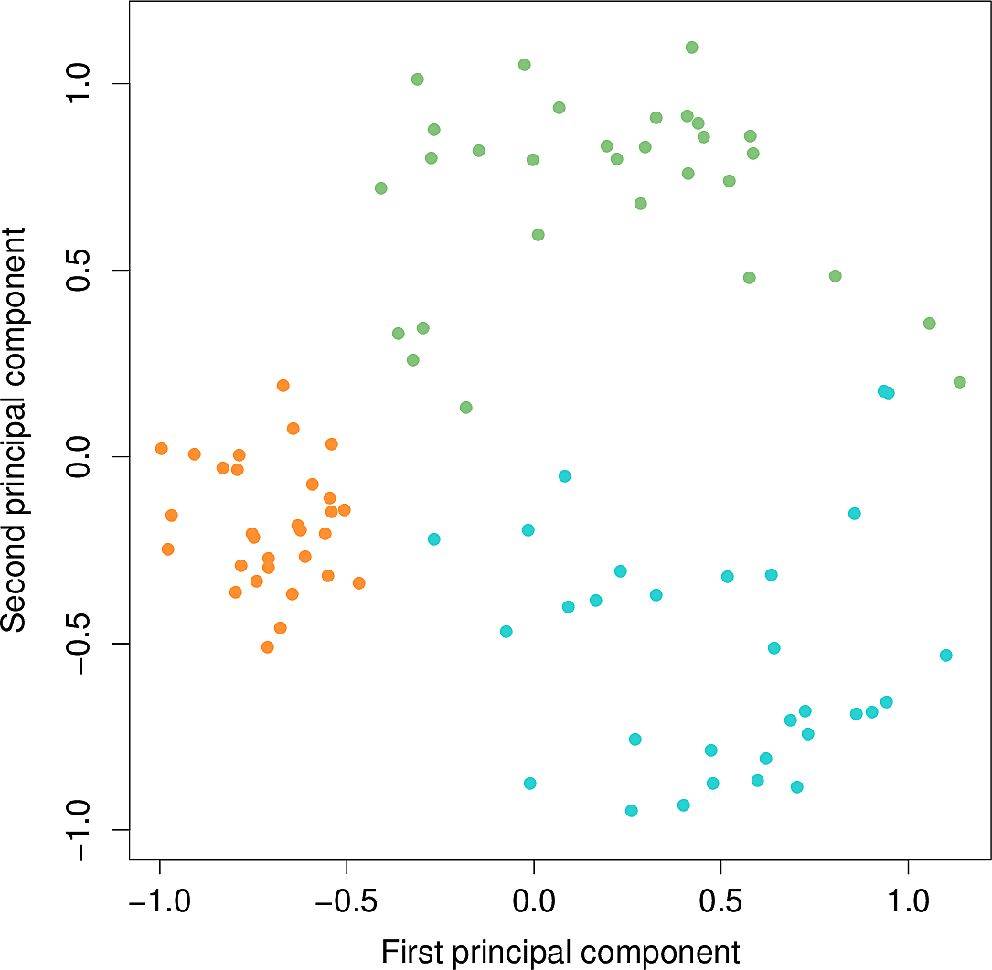
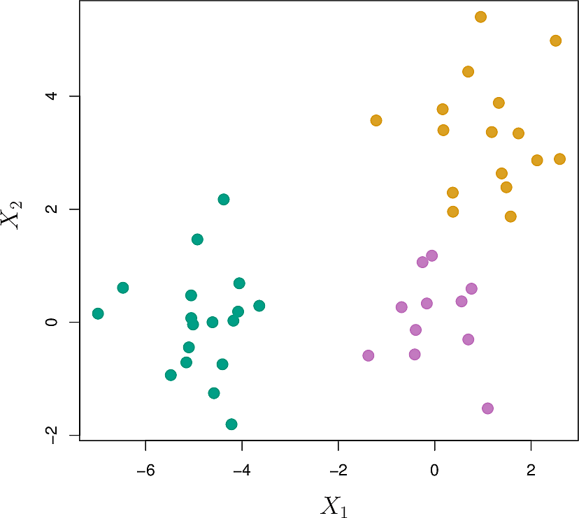
Let's look at a synthetic example generated from three classes.

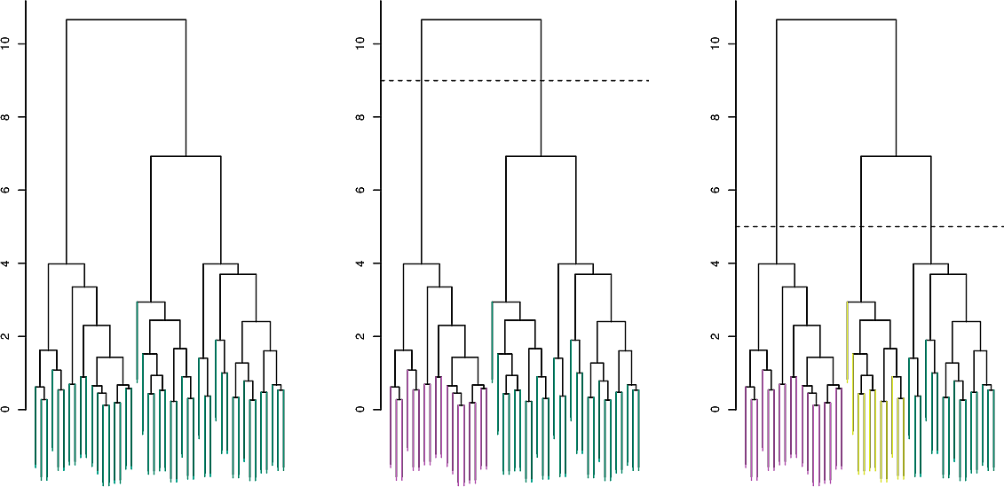
Hierarchical clustering yields the following dendrogram. By moving the dashed line up and down, we can select the number $K$ of clusters. This is often done by eye.

Note however that datasets do not always naturally lend themselves to hierarchical clustering. For example clustering AUC students with $K=3$ might be best done along the lines of student majors while $K=2$ might be best by gender.

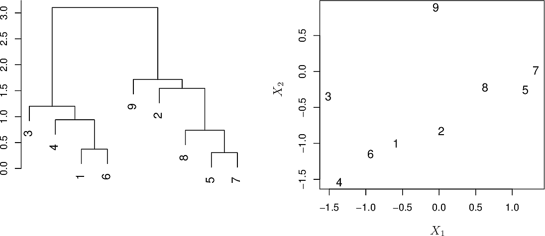
To see how similar two points are, we must consider the length of the path between them through the dendrogram, known as the cophenetic distance.

To cluster hierarchically, first determine a metric for inter-cluster distance, e.g the Euclidean distance between the centroids of the clusters.

Start by assigning each observation to its own cluster. Now computer the inter-cluster distances and fuse the two most similar clusters. Iterate until all observations are in a single cluster.

Several notions of inter-cluster distance, usually termed linkage, are used.

complete: the largest distance between elements of the two clusters
single: the smallest distance between elements of the two clusters
average: the average distance between elements of the two clusters
centroid: the distance between the centroids of the two clusters

Of these, centroid linkage is non-monotonic which can lead to ambiguity in the resulting dendrograms.

Each linkage leads to a dendrogram of a different shape.

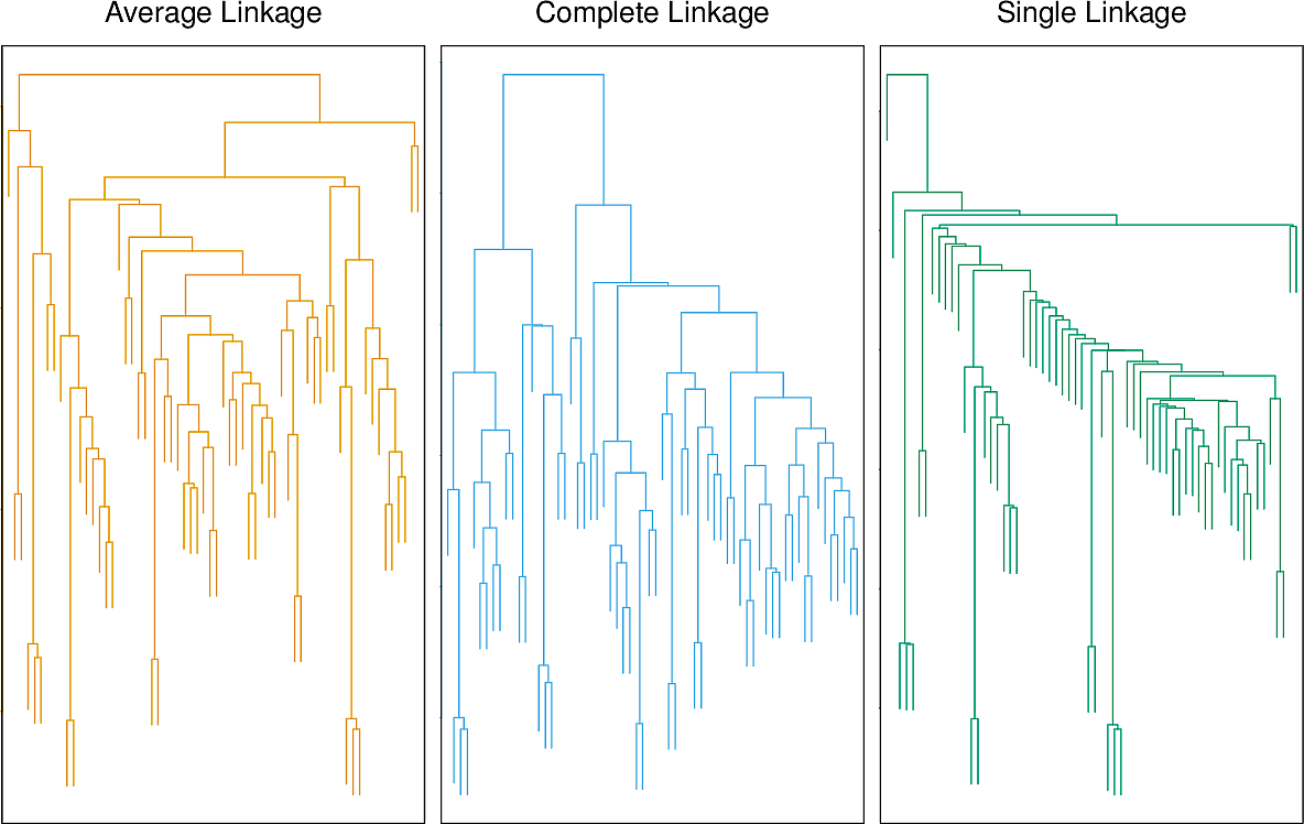
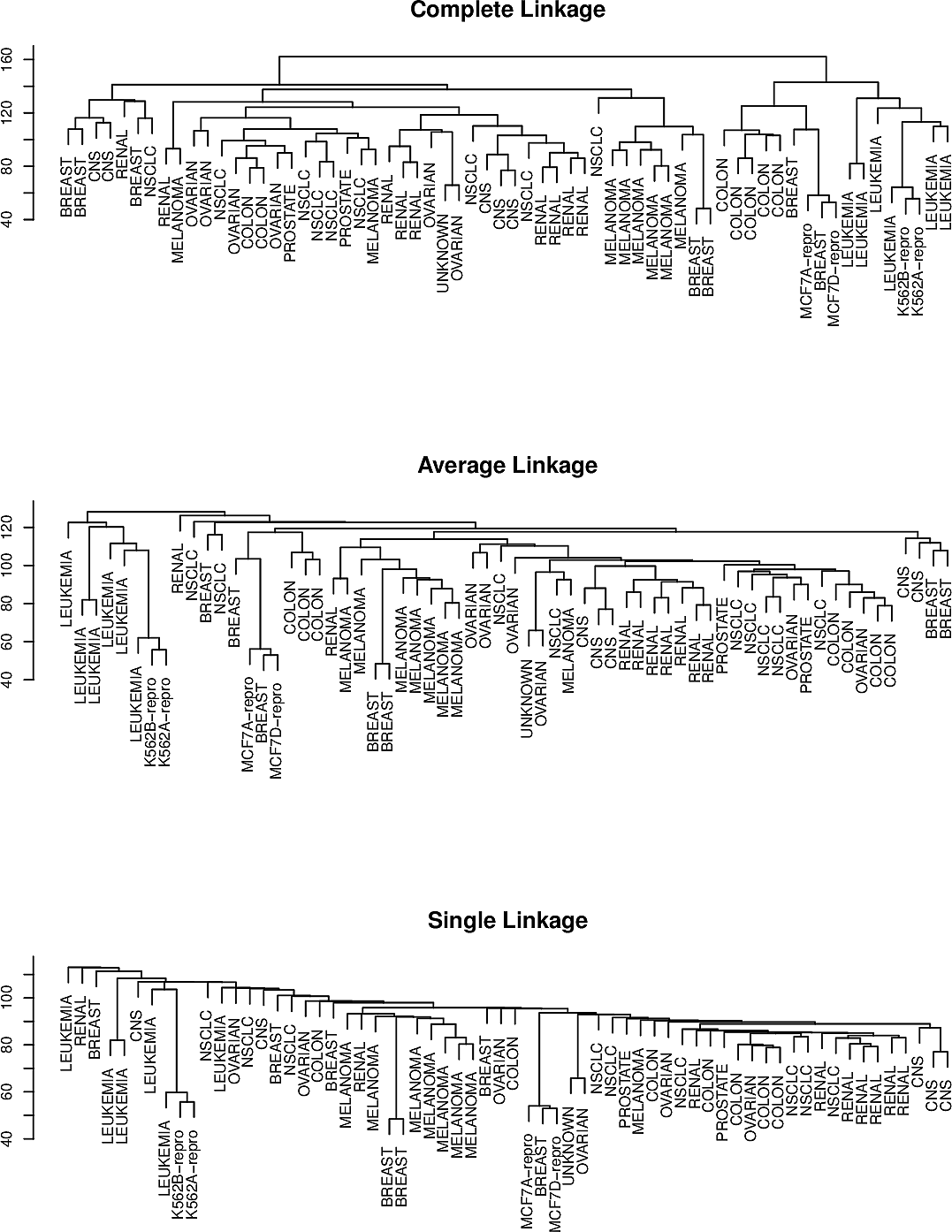
Many other cluster linkages are possible. Aside from distance-based linkages, correlation-based linkages have also been proposed.

Considerations

Clustering is subjective. Many decisions and judgements need to be made, each of which can have a large impact on the outcome. We say that clustering is not robust.

Should we standardize our data in some way before clustering?
Do we want to fix the number of clusters in advance?
Do the data lend themselves to hierarchical clustering?
What distance metric should we use?
What linkage should we use?
Where should we cut our dendrogram?

Often we cluster in order to carry out a further supervised learning task where we have a well defined performance metric. We can use this to select our clustering approach.

Sometimes clustering can force outliers into a cluster where they don't belong. Consider the "gendered" clustering above. This can lead to poor outcomes. Mixture models can be helpful here.

etc

Example exam 1 solution