Tree-based Methods
Exam 1 recap
Questions
- How was your experience of the exam?
- Were you surprised by anything in the exam description?
- In what ways did you feel you were well prepared for the exam?
- In what ways did you feel you were not well prepared for the exam?
- What went well?
- What went wrong?
- What did you spend more time on than you expected to?
- How much of your time did you spend on…
- coding
- debugging
- writing text
- looking up documentation
- searching for answers to questions
- interacting with LLMs
- other things
- How did you use LLMs?
- Which LLM(s) did you use?
- If you could go back in time three weeks, what would you have prepared better or practiced more?
- Do you think this is a fair way of examining this course?
- polars vs pandas
Feedback
- polars vs pandas
- It's not helpful to plot
median_house_valueandlongitudeon the same scale. Note
"\\mnt\\c\\Users\\98755\\Desktop\\Machine Learning"
or
r"\mnt\c\Users\98755\Desktop\Machine Learning"
Also with pathlib, can write with "/"
- 60 lines of imports, all used? ruff
- 400 LoC, 4 commits
Is there a better way to get numeric columns?
# Select numeric columns
numeric_cols = [
    col
    for col, dtype in zip(df.columns, df.dtypes)
    if dtype
    in (
        pl.Int8,
        pl.Int16,
        pl.Int32,
        pl.Int64,
        pl.UInt8,
        pl.UInt16,
        pl.UInt32,
        pl.UInt64,
        pl.Float32,
        pl.Float64,
    )
    and col != target
]
Try
df.select(cs.numeric())
LLMs
- Inaccessible links!
- for (NL) translation
- ask in your native language
- prep in advance
- review your work
priming
remember all of this information in the document! go thorugh it carefully and
remember the code, approaches and logic used. i will give you tasks to
solve/code later but only ever adapt code and use the the approaches that
were aready mentioned here! this is very important. if something is not
dicusses how to solve, then let me know that you don´t know from the document
how to solve it. remember tor prioritise polars over pandas
exam
Awesome — here’s an exam-ready starter that sticks exactly to your cheat-sheet + doc
- Overview. During the exam you depended a lot on ChatGPT, so much so that it appears
that you lost sight of what it was that you were doing. It would have been better to ask questions step by step. In that way you can keep the overview and help ChatGPT help you to solve your problems.
- Similarity mapping to previous exercises
- Good use of LLMs. Asked Claude and ChatGPR for feedback on code and report. I very much like this approach (and not only because the last part is doing my work for me!)
Data Ethics Project
Tree-based Methods
- We will look at tree-based methods for both classification and regression.
- Decision trees
- Sometimes called Classification and Regression Trees (CART)
- Two general techniques that are especially effective for combining decision
trees
- bagging
- boosting
Decision trees for apartments in NYC and SF


Decision trees for regression
We begin by building a decision tree for regression.
We use the Hitters data set of data on baseball players to predict their
Salary from the number of Years they have been playing and the number of
Hits they made in the previous year. Salaries are expressed as thousands of
dollars.
import polars as pl
from os import getenv
from pathlib import Path

import polars as pl
from dotenv import load_dotenv

load_dotenv(".envrc")

ISLP_DATADIR = Path(
    getenv("ISLP_DATADIR")
    or (
        "/home/bon/projects/auc/courses/ml/website/"
        "islp/data/ALL CSV FILES - 2nd Edition"
    )
)

hitters_csv = ISLP_DATADIR / "Hitters.csv"

hitters = pl.read_csv(hitters_csv)
hitters.shape
(322, 20)
Let's set the Polars print settings so that it does not elide the columns.
pl.Config.set_tbl_cols(-1)
pl.Config.set_tbl_width_chars(-1)
Let's have a look at the salaries.
hitters["Salary"]
shape: (322,)
Series: 'Salary' [str]
[
	"NA"
	"475"
	"480"
	"500"
	"91.5"
	…
	"700"
	"875"
	"385"
	"960"
	"1000"
]
It contains some NA values so the whole column is read as a string.
Let's try to read the csv file again, indicating that null values are
represented as NA in the file.
hitters = pl.read_csv(hitters_csv, null_values=["NA"])
hitters.dtypes
[Int64, Int64, Int64, Int64, Int64, Int64, Int64, Int64, Int64, Int64, Int64, Int64, Int64, String, String, Int64, Int64, Int64, Float64, String]
Now Salaries is Float64 with some nulls
import matplotlib.pyplot as plt

plt.clf()

bins = 32
plt.hist(hitters["Salary"], bins=bins)
plt.xlabel("salary")
plt.ylabel("frequency")
plt.savefig("images/hitters-salaries.png")
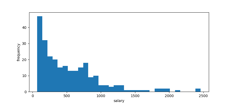
We see they are quite skewed and we suspect that such data are lognormally distributed. If this is so, then the logarithms of the data points will be normally distributed.
plt.clf()
plt.xlabel("log(salary)")
plt.ylabel("frequency")
plt.hist(hitters["Salary"].drop_nulls().log(), bins=bins)
plt.savefig("images/hitters-log-salaries.png")
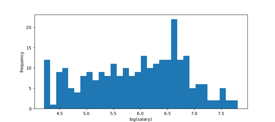
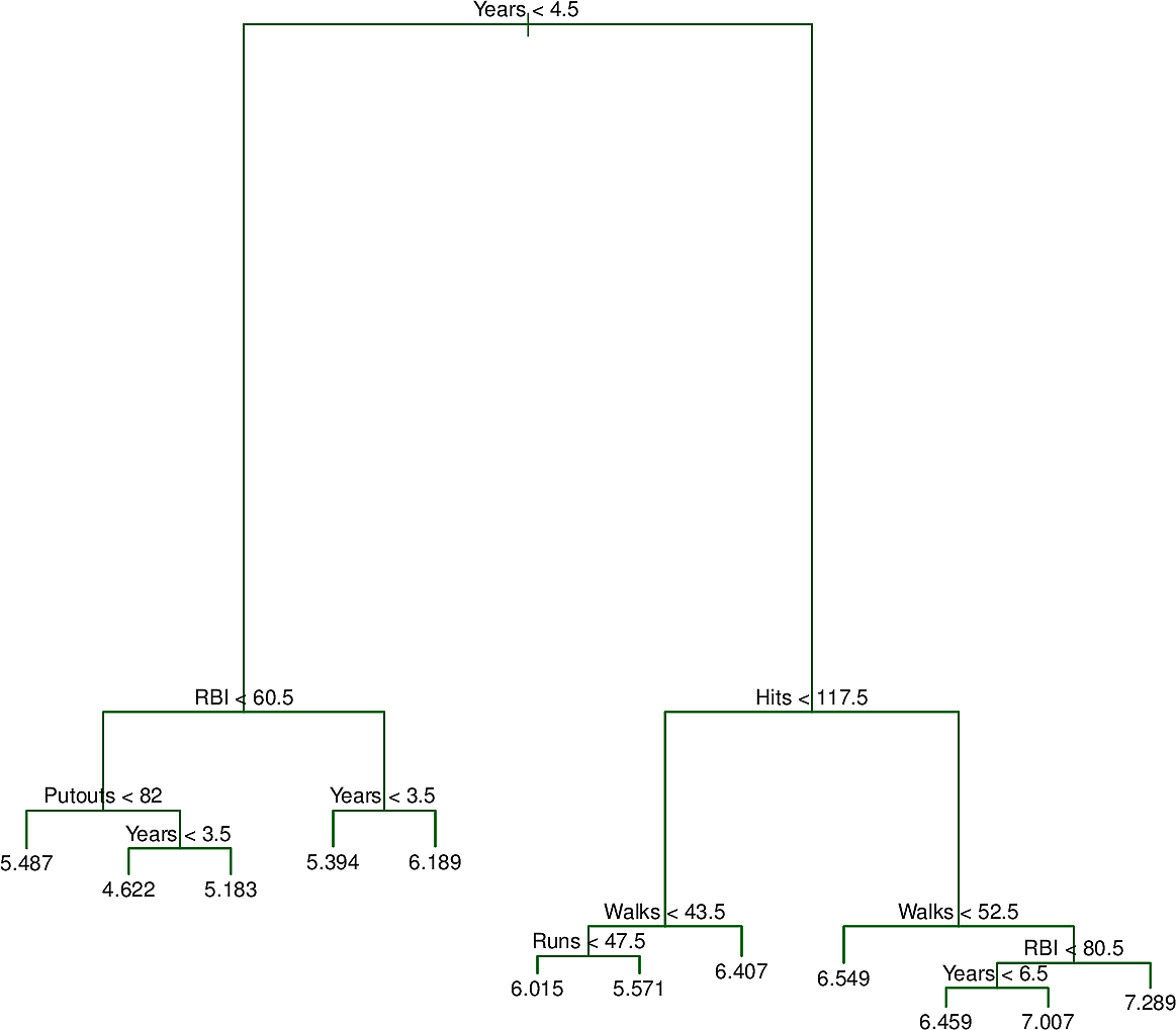
Now it does not look very normal but it is certainly less skewed so we will build a decision tree to predict LogSalary from Years and Hits. Here is an example of such a tree.
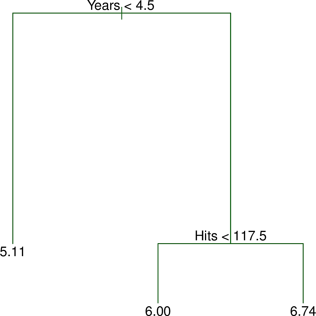
We note the following:
- Like many trees in computing, the tree is "upside down". Its root is at the top and its leaves are at the bottom.
- At the root is the decision \(Years < 4.5\). The training points for which this
is
truego to the left branch. The remaining points go to the right branch. - On the left is a leaf with the value \(5.11\), the mean of the salaries of all of the training points that have arrived there.
- On the right is another decision, \(Hits < 117.5\). Again the training points
for which this is
truego to the left branch while the remaining points go to the right branch. - The features
YearsandHitsare both of type integer. The splits are made half way between two integers. - For a new test data point, we start at the root and follow the decisions left and right until we reach a leaf. Then our prediction for
LogSalaryis the value at the leaf, e.g. \(5.11\) so our prediction forSalaryis then \(e^{5.11} \times 1000= \$165,670 \)
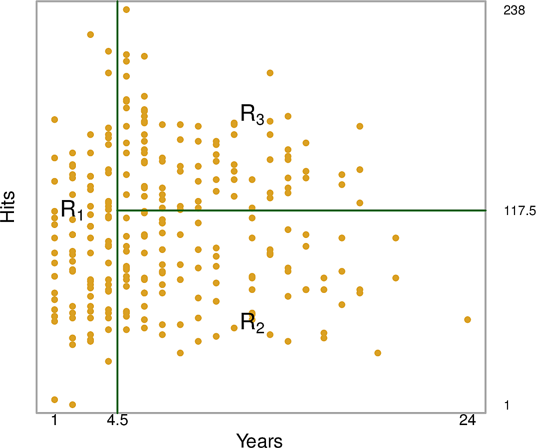
This tree partitions the training data points into three regions.
- \(R_1: Years < 4.5\)
- \(R_2: Years \geq 4.5 \wedge Hits < 117.5\)
- \(R_3: Years \geq 4.5 \wedge Hits \geq 117.5\)
The predictions for each of these regions are:
- \(R_1: \$165,670\)
- \(R_2: \$403,428\)
- \(R_3: \$845,561\)
We might interpret this as saying that the most important factor for predicting Salary is the number of Years played. For players with few Years, their previous year's number of Hits is less relevant but after 4 or 5 years, then it begins to play a role.
This might be an oversimplification but it has the advantage of being explainable.
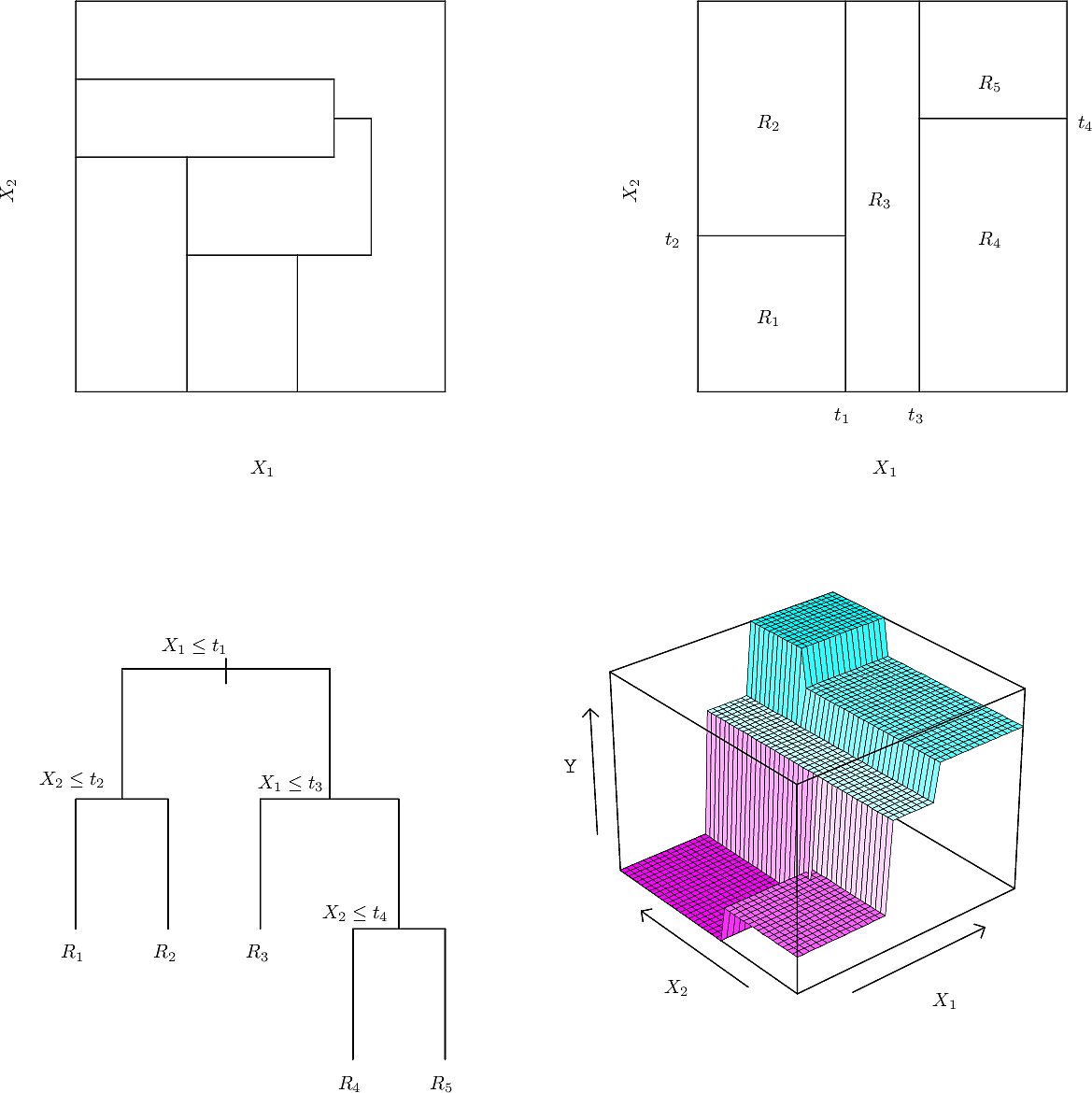
Stratification of the feature space
Now we take a step back and ask ourselves, of all of the partitions of the feature space, which one gives the best predictions? We can divide the process into two steps.
- We start with the \(p\) features \(X_1, \dots, X_p\). We split them into \(J\) non-overlapping regions, \(R_1, \dots, R_J\), which together cover the entire feature space. This is called a partition.
- For every observation that falls into region \(R_j\), we make the same prediction, namely the mean of the response values for the training points in \(R_j\).
Step 2 is straightforward but how about Step 1? Mathematically we seek to minimise the \(RSS\) given by: \[ RSS = \sum_{j=1}^J \sum_{i \in R_j} (y_i - \hat{y}_{R_j})^2 \]
But how can we choose from among all possible partitions, \(R_1, \dots, R_J\)? Its The computational complexity of finding the optimal partition is known to be NP-complete. This means that it is computationally intractable so we must use a heuristic approach. Many such approaches have been tried. Here we take the straightforward approach of recursive binary splitting. This is a top-down, greedy approach.
- top down
- means that we start at the root of our tree, which contains all of our training data, and split by branching.
- binary splitting
- means that each split divides the data at the tree node into two.
- greedy
- means that we make the best choice at each step before proceeding down the tree, rather than trying to look ahead and optimize over several steps.
At each step we select one predictor \(X_i\) and one value for \(X_i\) to split on, which we call the cutpoint \(s\), and then split the data points at the node into those for which \(X_i < s\), which we place to the left and those for which \(X_i \geq s\), which we place to the right. We examine all possible values of \(X_i\) and \(s\) and select the ones which lead to the greatest reduction in RSS.
We write \(\{X \mid X_i < s\}\) for the region in the \(p\)-dimensional space of predictors where \(X_i < s\).
Mathematically, we define the two half-planes
\begin{eqnarray*} R_l(i, s) &= \{X \mid X_i < s\} \\ R_r(i, s) &= \{X \mid X_i \geq s\} \\ \end{eqnarray*}and write \(\hat{y}_{R_l}\) and \(\hat{y}_{R_r}\) for the mean response in \(R_l(i, s)\) and \(R_r(i, s)\) respectively.
Then what we are looking for are the \(i\) and \(s\) which minimize \[ \sum_{k : \; x_k \in R_l(i, s)} (y_k - \hat{y}_{R_l})^ 2 + \sum_{k : \; x_k \in R_r(i, s)} (y_k - \hat{y}_{R_r})^ 2 \]
When \(p\) is not too large, we can find \(i\) and \(s\) quite quickly.
We iterate this process until we reach a stopping criterion. Examples of stopping criteria are:
- The node contains fewer than 8 data points
- All of the data points at the node have the same response (more usual for classification than regression). We say that a node is pure if all of its responses are the same. The impurity of a node is the extent to which its responses differ.
We will investigate some more sophisticated stopping criteria later.


Tree pruning
As we saw in the example of apartments in New York and San Francisco, if we continue too far with splitting we can overfit because our model becomes too complex.
We could prevent this by stopping once the reduction in RSS drops below a certain level. This could lead to a smaller tree which might generalise better.
However, since we are adopting a greedy approach, it might be that one step has a small reduction in RSS but the subsequent step has a larger reduction. To find such cases we first grow a large tree and then prune it.
But how should we prune it? Which subtree should we select? We should select the subtree with the lowest RSS. We could estimate this using cross validation. But again, just as with the original optimization problem, this too is intractable.
Rather than doing cross validation on every subtree, let's just "punish" the subtrees that are more complex, i.e. the bigger ones. Rather than looking for \(i\) and \(s\) which minimize \[ \sum_{k : \; x_k \in R_l(i, s)} (y_k - \hat{y}_{R_l})^ 2 + \sum_{k : \; x_k \in R_r(i, s)} (y_k - \hat{y}_{R_r})^ 2 \] let's add an extra term and minimize \[ \sum_{k : \; x_k \in R_l(i, s)} (y_k - \hat{y}_{R_l})^ 2 + \sum_{k : \; x_k \in R_r(i, s)} (y_k - \hat{y}_{R_r})^ 2 + \alpha \left| T \right| \]
Here \(\alpha\) is a number and \(\left| T \right|\) is the size of the subtree. In this way we punish the larger subtrees by giving them a higher cost and \(\alpha\) determines the degree to which we punish them. For \(\alpha=0\) there is no punishment while for a large \(\alpha\) larger subtrees are heavily punished.
(The idea of punishing more complex structures in general is known as regularization. We will see examples in other machine learning methods.)
To apply the pruning algorithm, call the quantity to be minimized, \(R(T)\) and initialize \(\alpha_1 = 0\) and \(T_1\) the tree which minimizes \(R(T)\).
Now iterate at step \(i\), writing \(T_t^i\) as the subtree of \(T\) at node \(t\) at iteration \(i\),
- Find \(t_i \in T^i\) which minimizes \(g_1(t) = { R(t) - R(T_t^i) \over \left| f(T_t^i) \right| -1 }\)
- Set \(\alpha_{i+1} = g_i(t_i)\) and \(T_{i+1} = T_i - T_{t_i}\)
This yields a sequence of subtrees \[ T^1 \supseteq T^2 \supseteq \dots \supseteq \text{root} \] and a sequence of alphas \[ \alpha_1 \leq \alpha_2 \leq \dots \leq \alpha_k \]
We choose the best \(\alpha_k\) by cross validation on testing data.
There are some worked examples here. We will do an example with scikit-learn .
Cost Complexity Pruning
This example, from the scikit-learn documentation, applies Cost Complexity Pruning to a data set on breast cancer for classification.
from sklearn.datasets import load_breast_cancer
from sklearn.model_selection import train_test_split
from sklearn.tree import DecisionTreeClassifier
We load the data and use cost_complexity_pruning_path to generate the paths, the alphas and the impurities.
X, y = load_breast_cancer(return_X_y=True)
X_train, X_test, y_train, y_test = train_test_split(X, y, random_state=0)

clf = DecisionTreeClassifier(random_state=0)
path = clf.cost_complexity_pruning_path(X_train, y_train)
ccp_alphas, impurities = path.ccp_alphas, path.impurities
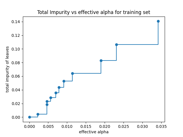
The final element is a tree with only a single node so we remove it and then plot how the value of \(\alpha\) effects impurity
fig, ax = plt.subplots()
ax.plot(ccp_alphas[:-1], impurities[:-1], marker="o", drawstyle="steps-post")
ax.set_xlabel("effective alpha")
ax.set_ylabel("total impurity of leaves")
ax.set_title("Total Impurity vs effective alpha for training set")
plt.savefig("images/impurities.png")
Now we train a decision tree on these alphas
clfs = [
    DecisionTreeClassifier(random_state=0, ccp_alpha=alpha).fit(
        X_train, y_train
    )
    for alpha in ccp_alphas
]
nodes = clfs[-1].tree_.node_count
ccp_alpha = ccp_alphas[-1]
f"Last tree has {nodes} node(s) and ccp_alpha: {ccp_alpha:0.4f}"
Last tree has 1 node(s) and ccp_alpha: 0.3273
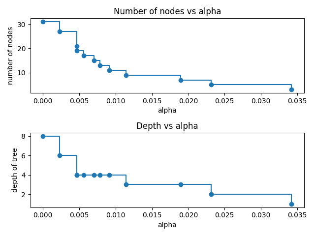
Let's remove those last elements and plot the number of nodes and the depth of the trees for the varying alphas.
clfs = clfs[:-1]
ccp_alphas = ccp_alphas[:-1]

node_counts = [clf.tree_.node_count for clf in clfs]
depths = [clf.tree_.max_depth for clf in clfs]
fig, ax = plt.subplots(2, 1)

ax[0].plot(ccp_alphas, node_counts, marker="o", drawstyle="steps-post")
ax[0].set_xlabel("alpha")
ax[0].set_ylabel("number of nodes")
ax[0].set_title("Number of nodes vs alpha")

ax[1].plot(ccp_alphas, depths, marker="o", drawstyle="steps-post")
ax[1].set_xlabel("alpha")
ax[1].set_ylabel("depth of tree")
ax[1].set_title("Depth vs alpha")

fig.tight_layout()
plt.savefig("images/tree_depths.png")
Finally let us see how the accuracy of our model on the training and test sets varies with \(\alpha\)
train_scores = [clf.score(X_train, y_train) for clf in clfs]
test_scores = [clf.score(X_test, y_test) for clf in clfs]

fig, ax = plt.subplots()

ax.set_xlabel("alpha")
ax.set_ylabel("accuracy")
ax.set_title("Accuracy vs alpha for training and testing sets")

common = {"marker": "o", "drawstyle": "steps-post"}
ax.plot(ccp_alphas, train_scores, label="train", **common)
ax.plot(ccp_alphas, test_scores, label="test", **common)
ax.legend()
plt.savefig("images/tree_accuracies.png")
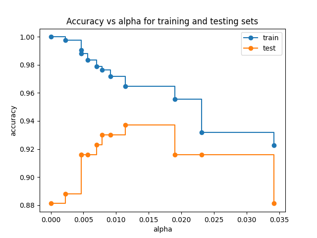
We see the familiar pattern of a continuing drop in training accuracy but a clear maximum in test accuracy at around \(\alpha = 0.015\)
Pruning the Hitters dataset
Here is an as yet unpruned tree for the Hitters dataset.
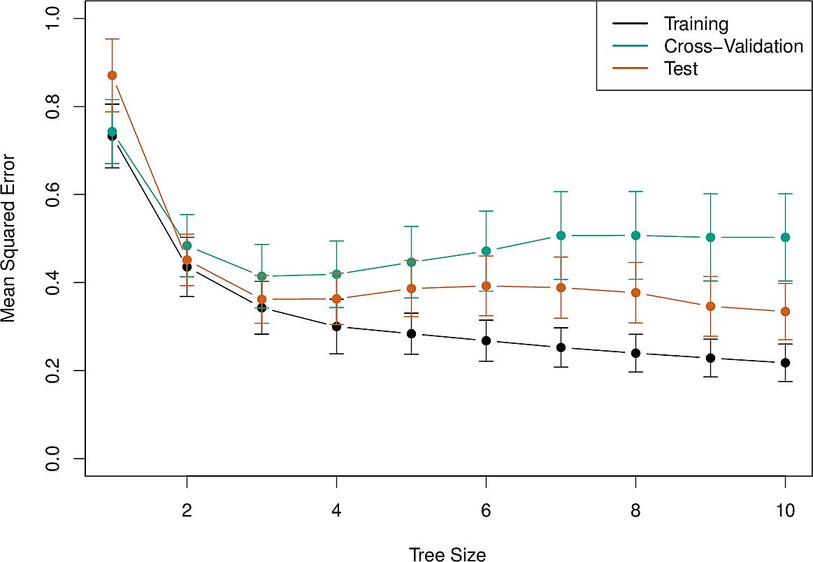
And here is an error analysis on training data, test data and cross-validation. The original dataset was split in two to form the training and test sets and cross-validation was done sixfold.
The pruned tree with three nodes is the one shown at the top of this section.
Decision trees for classification
Using decision trees for classification is very similar to using them for regression. We just need to make several tweaks.
Response
For regression, we used the mean for the response for each node. For classification we will use the most common response at the node.
Split function
classification error rate
For regression we used RSS to make binary splits. For classification we use the classification error rate \[ E = 1 - \max_k (\hat{p}_{mk}) \] where \(\hat{p}_{mk}\) is the ratio of training observations in region \(m\) that are from class \(k\).
It turns out that classification error rate is not sensitive enough for our purposes so two other splitting functions are commonly used.
Gini index
The Gini index, defined by \[ G = \sum_{k=1}^K \hat{p}_{mk} (1 - \hat{p}_{mk}) \] is also commonly used as an indicator of wealth inequality.
If most values of \(\hat{p}_{mk}\) are close to 0 or 1, then \(G\) is low. The Gini index is often described as a measure of node purity.
Entropy
An Information Theoretic measure closely related to the Gini index is Entropy, defined in our terms as \[ D = - \sum_{k=1}^K \hat{p}_{mk} \log \hat{p}_{mk} \] Similar to the Gini index, entropy takes on values close to zero when most values of \(\hat{p}_{mk}\) are close to 0 or 1 and in fact both measures behave similarly.
Of the three measures, experience shows that Gini or entropy tend to be better for splitting, whereas classification error rate works best for pruning.
Here is an example of the Heart dataset (not documented in the ISLP
documentation) consisting of 303 patients who presented with chest pain. There
are 13 predictors of whether an angiographic test would indicate the presence
of heart disease. This is thus a classification task with a Yes/No outcome.
Furthermore this dataset has categorical predictors. This does not present a problem to us since we can split on a predictor having one of the values as against the other possible values.
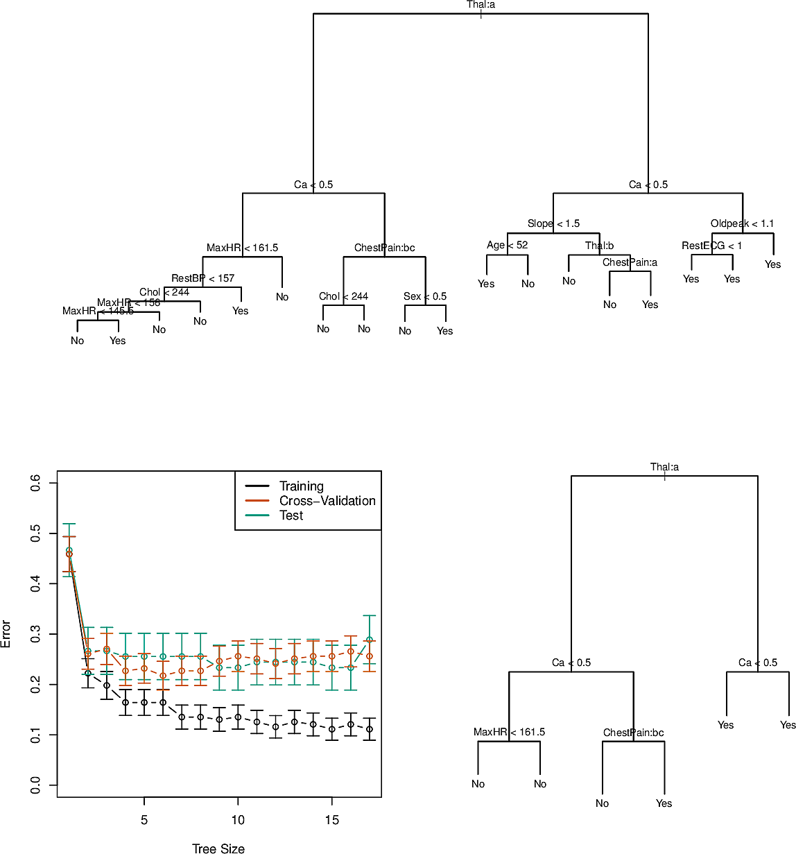
Something that might appear strange at first glance is that there are nodes which split to two child nodes which have the same predicted value, e.g. the node with RestEGC < 1 has Yes at both children. This is because of node purity. The leaf node on the left has \(7/11\) observed data points with Yes, whereas the node on the right has all \(9\) as Yes. We can thus be more confident of a Yes for a RestEGC greater than \(1\). So this split does nothing to improve the classification error but it does improve our confidence in some cases.
Tree-based models vs Linear models
Tree-based models and Linear models are very different in nature. What are their advantages and disadvantages?
Advantages of tree-based models
They are easily explainable. There has been a great deal of attention in recent years for explainable AI, with ethical questions being asked about black-box systems which can be understood by neither laypersons nor experts.
In the EU, the Right to Explanation is a cornerstone of the GDPR.
- They are considered more natural and similar to human reasoning.
- They can be displayed graphically which aids visual thinking.
- They can easily cater for categorical variables.
- They require very little preprocessing.
- Feature importance can be easily derived from a decision tree.
- They can be made robust against colinearity.
Disadvantages of tree-based models
- They do not always reach the levels of predictive accuracy of other modelling approaches.
- They are not very robust, with small changes in the input data sometimes giving very different results.
- Learning an optimal decision tree is NP-complete so we need to use heuristics.
However, there are techniques which can mitigate these disadvantages to some degree.
Ensemble Methods
An ensemble method is an approach which combines other weaker methods into a stronger machine-learning method. We investigate several approaches to making ensembles of tree-based methods.
Bagging
In an earlier class we looked at The bootstrap as a way of getting a better estimate of a values when the variance is high. Decision trees also suffer from high variance so we can use a kind of bootstrap known as bootstrap aggregation or bagging.
We saw that if we take \(n\) samples \(Z_1, Z_2, \dots, Z_n\), each with variance \(\sigma^2\), then the variance on the mean \(\bar{Z}/n\) will be \(\sigma^2/n\).
When building decision trees we can also bootstrap \(B\) different training sets and average their predictors. We grow the trees deep without pruning. As a result they have high variance but combining hundreds or even thousands of them by bagging can significantly improve accuracy.
For regression we average the predictions. For classification we use majority vote.
An interesting byproduct of the way bagging is done is that about 2/3 of the data points are chosen for each bootstrap sample. The fraction is actually given by \[ 1 - \frac{1}{e} = 0.6321 \] This means that we have about 1/3 of the data points available for validation. These are called the out-of-bag (OOB) data points. So instead of having to make a test set or do cross-validation, we have a read made set of points to test on.
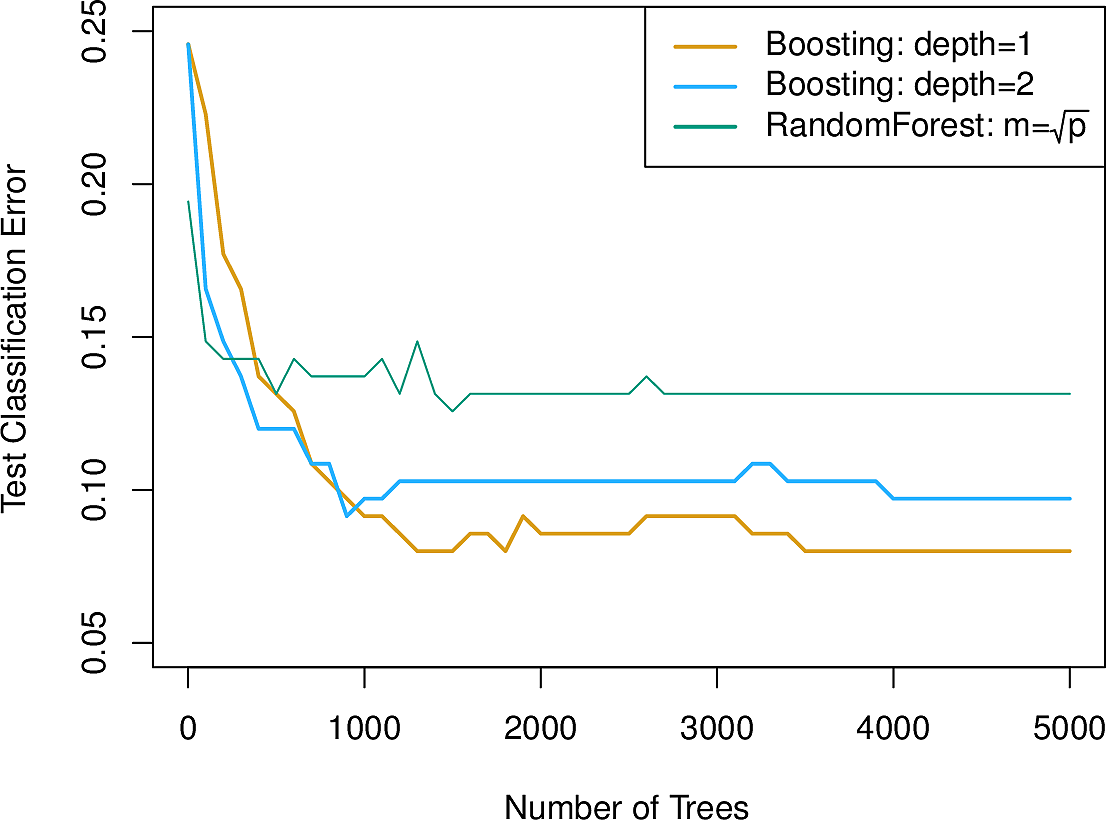
Here is a comparison of several of these approaches for the Heart data set.
We see that bagging with a test set improves on a decision tree (the dashed
line) and that OOB improves upon that. Random forests make a further
improvement.

Random forests
Random forests are decision trees with bagging with a refinement. Instead of considering all \(p\) features when splitting at a node, we consider only a sample of \(m \approx \sqrt{p}\) of them.
This has the advantage of bringing more diversity to the trees generated. Without sampling, if there are several strong predictors among the features they will almost always get selected for splitting and the resulting trees will be highly correlated. With sampling, the other features are chosen more often and the correlation will be less. It decorrelates the trees.
We can see in the previous figure how this improves the errors.
The hyperparameter \(m\) can be adjusted depending on the data set. For a data set with a large number of features, many of which are correlated, it can be useful to take an even smaller \(m\).
The NCI 60 dataset contains high-dimensional biological data. The goal was to predict one of 14 cancer types based on gene expression. In the plot we see that 100 or so trees gives good performance and that random forests with \(m \approx \sqrt{p}\) improves on plain bagging (\(m = p\)).
Boosting
Boosting is another way in which we can improve decision trees. It is a general approach that can be applied to other methods of machine learning. While bagging takes a number of independent samples, boosting generates a sequence of trees where each one is generated from the previous one. Instead of immediately fitting a deep tree, we deliberately keep the trees small. We fit a first tree to the outcome \(y\) and then fit each subsequent tree to the residuals of the previous tree. In this way we seek to improve our tree in areas where it does not perform well. The idea is to learn slowly. The algorithm for regression is as follows.
- Initialize by setting \(\hat{f}(x) = 0\) and \(r_i = y_i\) for each \(i\) in the training set.
- For \(b \in 1,2,\dots,B\)
- Fit a tree \(\hat{f}_b\) with \(d\) splits to the training data \((X, r)\).
- Shrink \(\hat{f}\) by \(\hat{f}(x) \leftarrow \hat{f}(x) + \lambda \hat{f}_b(x)\)
- Update the residuals \(r_i \leftarrow r_i - \lambda \hat{f}_b(x_i)\)
- The boosted model is \[ \hat{f}(x) \sum_{b=1}^B \lambda \hat{f}_b(x) \]
Note that there are three hyperparameters to tune.
- \(B\)
- the number of trees
- \(\lambda\)
- the shrinkage parameter, a kind of learning rate, typically \(10^{-2}\) or \(10^{-3}\)
- \(d\)
- the number of splits in each tree, which can be as low as 1 for an additive model or, more generally is known as the interaction depth.
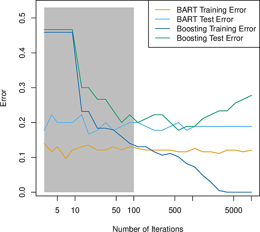
Here is boosting applied to the previous cancer data set. We see that it slightly outperforms random forests. As it produces a sum of smaller trees, this can aid explainability.
Bayesian Additive Regression Trees
Bayesian Additive Regression Trees (BART) combine the advantages of bagging and boosting by taking elements from both. As in boosting, a succession of trees is constructed, each using bagging, and each focusing on capturing signal not yet accounted for.
We consider regression.
At each of the \(B\) iterations we will have \(K\) trees. We write \(\hat{f}_k^b(x_i)\) for the prediction at \(x_i\) by tree \(k\) on iteration \(b\). After each iteration, we sum the \(k\) trees from that iteration. \[ \hat{f}^b(x) = \sum_{k=1}^K \hat{f}^b_k(x) \]
At each iteration BART randomly perturbs the tree in one of several ways looking for variations that improve the fit. For example the following tree:
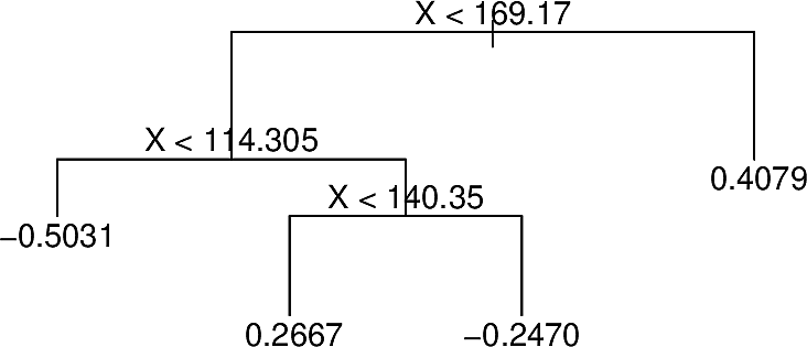
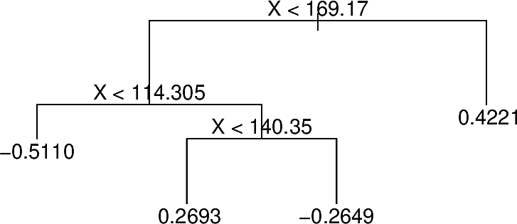
With different predictions at some terminal nodes
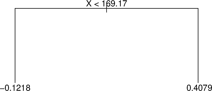
After pruning
With terminal nodes added
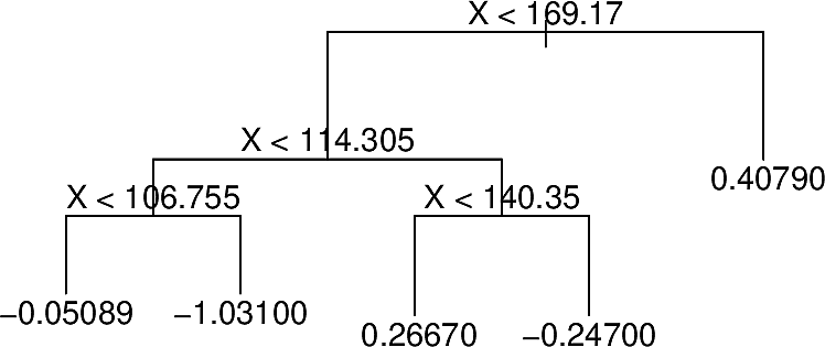
These perturbations server to increase the diversity of the trees.
Another feature of BART is the employment of a burn-in period. The trees
generated in early iterations are often of low quality and do not contribute to
a good final model so they are not included. Typically several hundred
iterations are excluded. Here we see BART on the Heart data settling down
after a burn-in period.
Variable importance measures
When we have a single decision tree, it is easy by inspection to see which features are more important than others. In methods such as bagging, where we have many trees, this can be less obvious.
We can however look at how many times nodes were split on each feature and what the total reduction in RSS was. In this way we can get a measure of variable importance.

Decision Trees from Scratch
This material adapted from Machine Learning from Scratch by Marvin Lanhenke

from sklearn import datasets
from sklearn.model_selection import train_test_split
import numpy as np
class Node:
    def __init__(
        self,
        feature=None,
        threshold=None,
        left=None,
        right=None,
        *,
        value=None
    ):
        self.feature = feature
        self.threshold = threshold
        self.left = left
        self.right = right
        self.value = value

    def is_leaf(self):
        return self.value is not None
class DecisionTree:
    def __init__(self, max_depth=100, min_samples_split=2):
        self.max_depth = max_depth
        self.min_samples_split = min_samples_split
        self.root = None

    def _is_finished(self, depth):
        return (
            depth >= self.max_depth
            or self.n_class_labels == 1
            or self.n_samples < self.min_samples_split
        )

    def _entropy(self, y):
        proportions = np.bincount(y) / len(y)
        entropy = -np.sum([p * np.log2(p) for p in proportions if p > 0])
        return entropy

    def _create_split(self, X, thresh):
        left_idx = np.argwhere(X <= thresh).flatten()
        right_idx = np.argwhere(X > thresh).flatten()
        return left_idx, right_idx

    def _information_gain(self, X, y, thresh):
        parent_loss = self._entropy(y)
        left_idx, right_idx = self._create_split(X, thresh)
        n, n_left, n_right = len(y), len(left_idx), len(right_idx)

        if n_left == 0 or n_right == 0:
            return 0

        child_loss = (n_left / n) * self._entropy(y[left_idx]) + (
            n_right / n
        ) * self._entropy(y[right_idx])
        return parent_loss - child_loss

    def _best_split(self, X, y, features):
        split = {"score": -1, "feat": None, "thresh": None}

        for feat in features:
            X_feat = X[:, feat]
            thresholds = np.unique(X_feat)
            for thresh in thresholds:
                score = self._information_gain(X_feat, y, thresh)

                if score > split["score"]:
                    split["score"] = score
                    split["feat"] = feat
                    split["thresh"] = thresh

        return split["feat"], split["thresh"]

    def _build_tree(self, X, y, depth=0):
        self.n_samples, self.n_features = X.shape
        self.n_class_labels = len(np.unique(y))

        # stopping criterion
        if self._is_finished(depth):
            most_common_Label = np.argmax(np.bincount(y))
            return Node(value=most_common_Label)

        # get best split
        rnd_feats = np.random.choice(
            self.n_features, self.n_features, replace=False
        )
        best_feat, best_thresh = self._best_split(X, y, rnd_feats)

        # grow children recursively
        left_idx, right_idx = self._create_split(X[:, best_feat], best_thresh)
        left_child = self._build_tree(X[left_idx, :], y[left_idx], depth + 1)
        right_child = self._build_tree(
            X[right_idx, :], y[right_idx], depth + 1
        )
        return Node(best_feat, best_thresh, left_child, right_child)

    def _traverse_tree(self, x, node):
        if node.is_leaf():
            return node.value

        if x[node.feature] <= node.threshold:
            return self._traverse_tree(x, node.left)
        return self._traverse_tree(x, node.right)

    def fit(self, X, y):
        self.root = self._build_tree(X, y)

    def predict(self, X):
        predictions = [self._traverse_tree(x, self.root) for x in X]
        return np.array(predictions)
def accuracy(y_true, y_pred):
    return np.sum(y_true == y_pred) / len(y_true)


data = datasets.load_breast_cancer()
X, y = data.data, data.target

X_train, X_test, y_train, y_test = train_test_split(
    X, y, test_size=0.2, random_state=1
)

clf = DecisionTree(max_depth=10)
clf.fit(X_train, y_train)

y_pred = clf.predict(X_test)
acc = accuracy(y_test, y_pred)

f"Accuracy: {acc:0.4f}"
Accuracy: 0.9561