Generative Models for Classification
Bayes rule
For classification we seek to model \(Pr(Y=k | X=x)\), in other words, the probability that the response is in class \(k\) when the predictor is \(x\).
The Logistic Regression method models this probability as a logistic function.
Now let's look at each of the response classes separately and for each one
model the distribution of the corresponding \(X\). So, for example, in the
Smarket data we separate out the lines where Direction is Up and those
where Direction is Down.
For certain kinds of data sets this approach has advantages over logistic regression:
- When the classes are separated logistic regression can be unstable
- When the distributions of \(X\) are well modelled by a normal distribution
- They extend naturally to cases where there are more than two classes.
Let's consider \(K\) classes where \(K \geq 2\).
Write \(\pi_k\) for the probability that a randomly chosen observation is in class \(k\). We call this the prior probability.
Considering all the observations in class \(k\), we write their distribution as \[ f_k(X) = Pr(X | Y=k) \]
Now Bayes' theorem allows us to flip that expression to get \[ p_k(x) = Pr(Y=k | X=x) = { \pi_k f_k (x) \over \sum_{i=1}^K \pi_i f_i(x) } \]
We call \(p_k(x)\) the posterior probability.
Now if we can estimate each of the \(\pi_k\) and \(f_k\) then can get an estimate for \(p_k\).
Estimating \(\pi_k\) is easy from a sample; it's just the relative number of observations in each class.
Estimating the \(f_k\) can be trickier; we often need to make extra, simplifying assumptions. We look at three approaches.
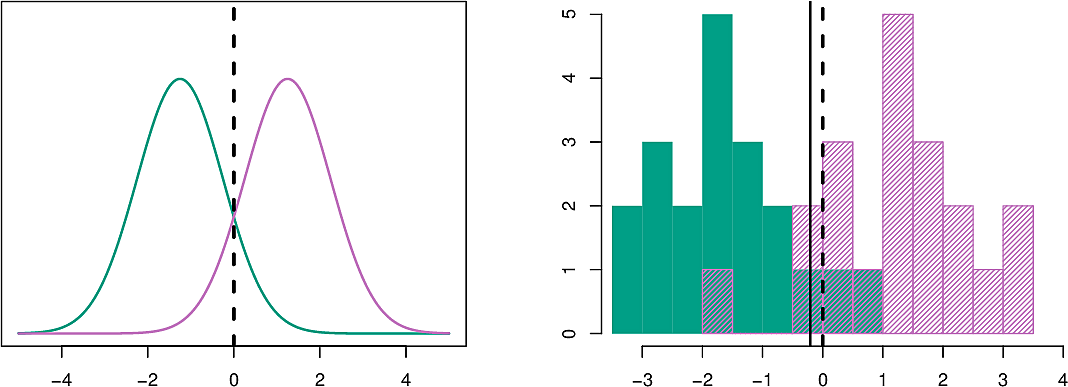
Linear Discriminant Analysis (\(p=1\))
We consider only one predictor, \(p=1\), and assume \(f_k\) is distributed normally. \[ f_k(x) = { 1 \over \sqrt{2\pi} \sigma_k } \exp \left( - { 1 \over 2 \sigma_k^2 } (x - \mu_k)^2 \right) \]
We make the further assumption that all of the \(\sigma_k^2\) are equal, i.e. \[ \sigma_1^2 = \sigma_2^2 = \ldots = \sigma_K^2 \]
The Bayesian Classifier now assigns an observation \(x\) to the class \(k\) for which \(f_k(x)\) is the largest.
Linear Discriminant Analysis approximates the Bayes classifier by estimating the \(\pi_k\), \(\mu_k\) and \(\sigma\), the latter being the weighted average of the sample variances of each of the \(k\) classes.
In the figure on the left we see two normal distributions with the Bayes boundary between them. On the right, two samples shown as histograms. The Bayes boundary is the midpoint between the two sample means.
Linear Discriminant Analysis (\(p>1\))
The approach extends straightforwardly to a multivariate normal distribution with a common covariance matrix and a class-specific mean. \[ f_X(\mathbf{x}) = { \exp \left( - \frac{1}{2} (\mathbf{x} - \mathbf{\mu})^T \Sigma^{-1} (\mathbf{x} - \mathbf{\mu}) \right) \over \sqrt{(2\pi)^{p/2} \left| \Sigma \right|^{1/2}}} \] where \(p\) is the number of predictors and \(k\) is the number of classes.
Here are examples of such distributions. On the left a symmetric one with \(Var(X_1) = Var(X_2)\) and \(Cov(X_1, X_2) = 0\) and on the right one with different variances and a correlation between the variables.
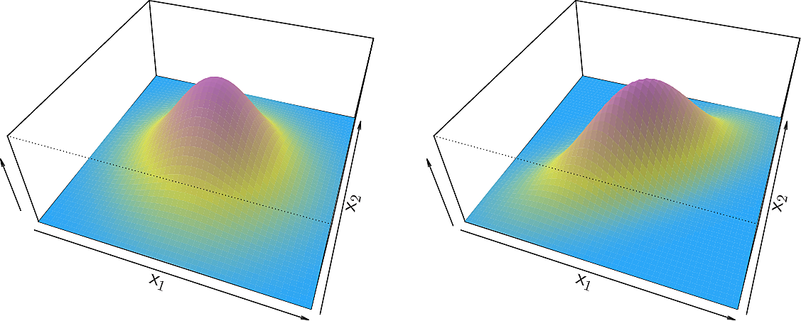
Similarly to the one-dimensional LDA, here we estimate \(\pi_k\), \(\mathbf{\mu}_k\) and \(\mathbf{\Sigma}\)
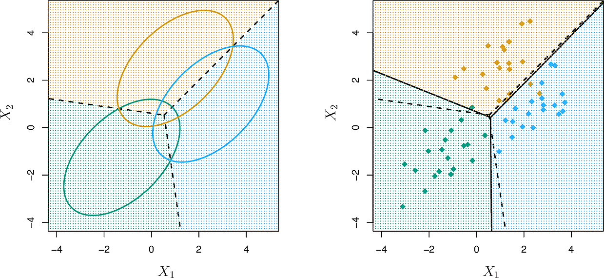
Here is an example of 3 classes over 2 predictors. On the left, the ellipses contain 90% of the probability mass of each multivariate normal distribution. The dashed lines are the Bayesian decision boundaries. On the right, 20 observations are drawn from each class. The LDA boundaries are shown as solid black lines.
Let's look at the confusion matrix for LDA on the Default dataset.
| True No | True Yes | Total | |
|---|---|---|---|
| Predicted No | 9644 | 252 | 9896 |
| Predicted Yes | 23 | 81 | 104 |
| Total | 9667 | 333 | 10000 |
- The model predicts many of the defaults (81) and non-defaults (9644).
- Only 23 people who did not default were predicted to do so.
- Of the 333 who defaulted, the model only predicted 81 (24.3%).
- Should we be more worried about the false positives or false negatives? See e.g. the Dutch childcare benefits scandal
The following quantities are often used in medicine:
- sensitivity
- percentage of defaulters correctly identified
- specificity
- percentage of non-defaulters correctly identified
We can improve the results of our classifier by moving its thresholds. Where we had identified a default when
\[
Pr(\mathtt{default} = \mathtt{Yes}) | X = x) > 0.5
\]
we will catch more defaults if we use the threshold
\[
Pr(\mathtt{default} = \mathtt{Yes}) | X = x) > 0.2
\]
Now our confusion matrix looks like this.
| True No | True Yes | Total | |
|---|---|---|---|
| Predicted No | 9432 | 138 | 9570 |
| Predicted Yes | 235 | 195 | 430 |
| Total | 9667 | 333 | 10000 |
Now it correctly predicts 195 of those who defaulted (59%), a significant improvement. However we now predict 12 fewer non-defaults correctly but we may consider this a reasonable price to pay.
We can look at how moving the threshold effects both the fraction of defaulting clients misclassified (in blue) as well as the error rates, overall (in black) and among the non-defaulting clients (in orange).
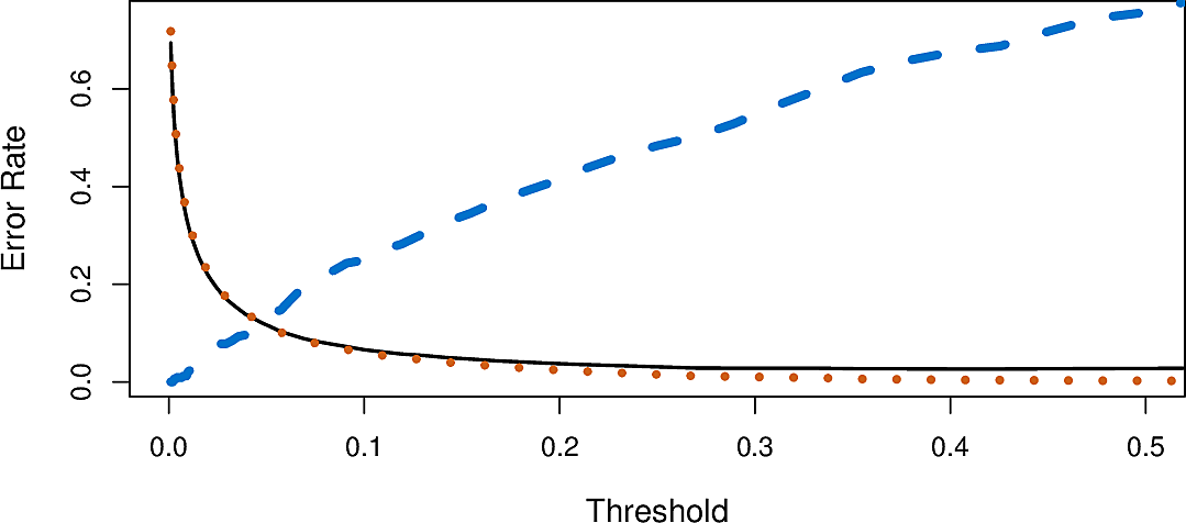
The decision on which threshold to accept is a business decision, depending on domain knowledge, and ultimately comes down to the value added by the model.
ROC Curve
A Receiver operating characteristic (ROC) curve was originally developed by radar engineers during the last world war. It is a means of graphing two types of error across a range of thresholds. The false-positive rate is plotted on the x-axis with the false-negative rate on the y-axis.
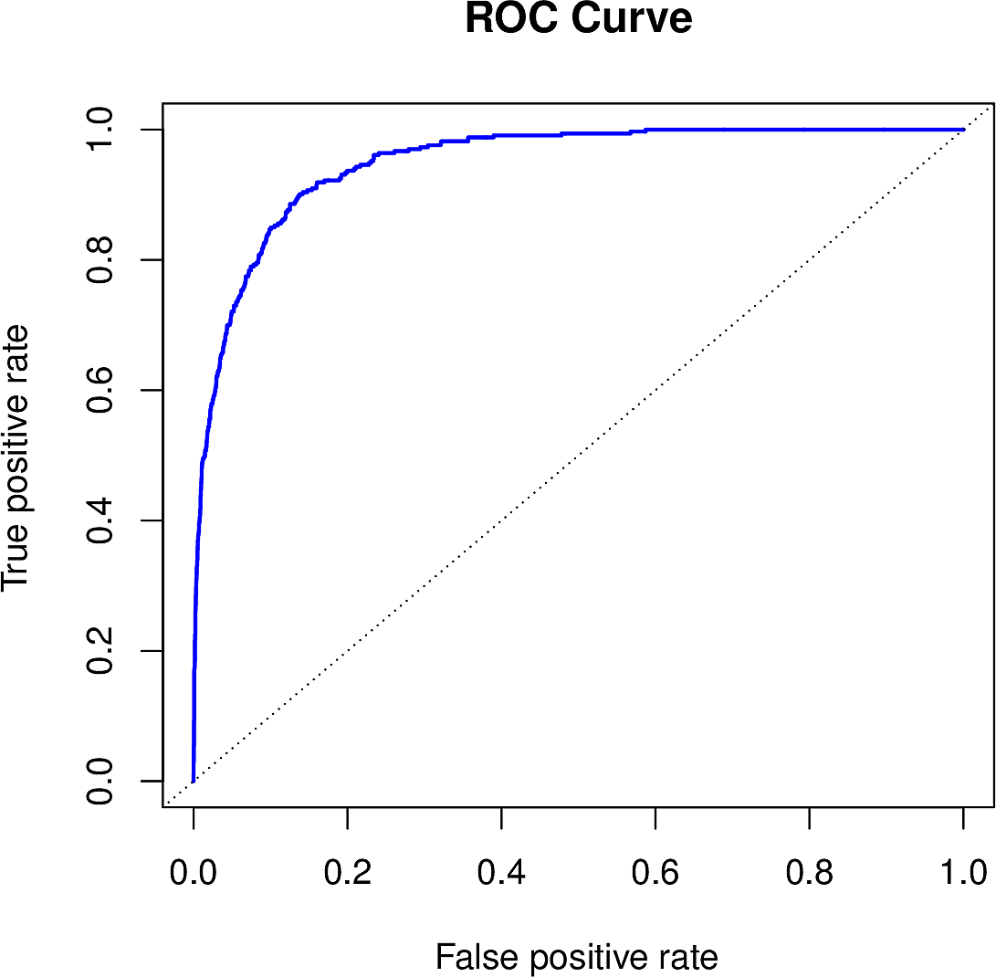
The closer the ROC curve is to the top left corner, the better the classifier.
The diagonal line represents the ignorant classifier. In this way the ROC curve
can be used to compare classifiers by calculating the area under the curve
(AUC). The AUC for LDA on the Default data is 0.95, a high value.
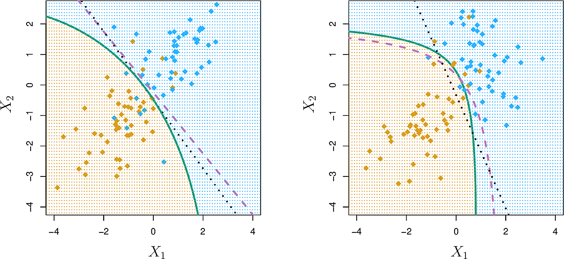
Quadratic Discriminant Analysis
If we take LDA and drop the requirement that each class have the same covariance matrix, we get Quadratic Discriminant Analysis (QDA). This approach is somewhat more complex since we now need to estimate more parameters. For \(p\) predictors, there are \(Kp(p+1)/2\) parameters, whereas for LDA there are only \(Kp\).
This can lead to improved prediction performance but can also lead to high bias if the assumption about the covariance matrix is not warranted.