Classification

The regression problems we studied so far have a response variable that is quantitative, i.e. a number. Now we switch to looking at problems where the response variable is qualitative. We call such variables categorical.

Here are some categorical variables we might like to predict

eye colour: from genetic data
fraudulent credit-card payments: from transaction history, time and place of payment, payment amount and goods or services bought
medical conditions: from symptoms and patient medical history and demographic
deleterious DNA mutations: from sequence data and epidemiological data on patients

Whereas predicting quantitative variables is known as regression, predicting quanlitative variables is known as classification. We aim to predict whether a given observation belongs to one of a number of classes or categories.

Doing so might involve predicting the probabilities that the observation belongs to each category and then choosing the category with the highest probability. In this sense, classification reduces to a number of regressions.

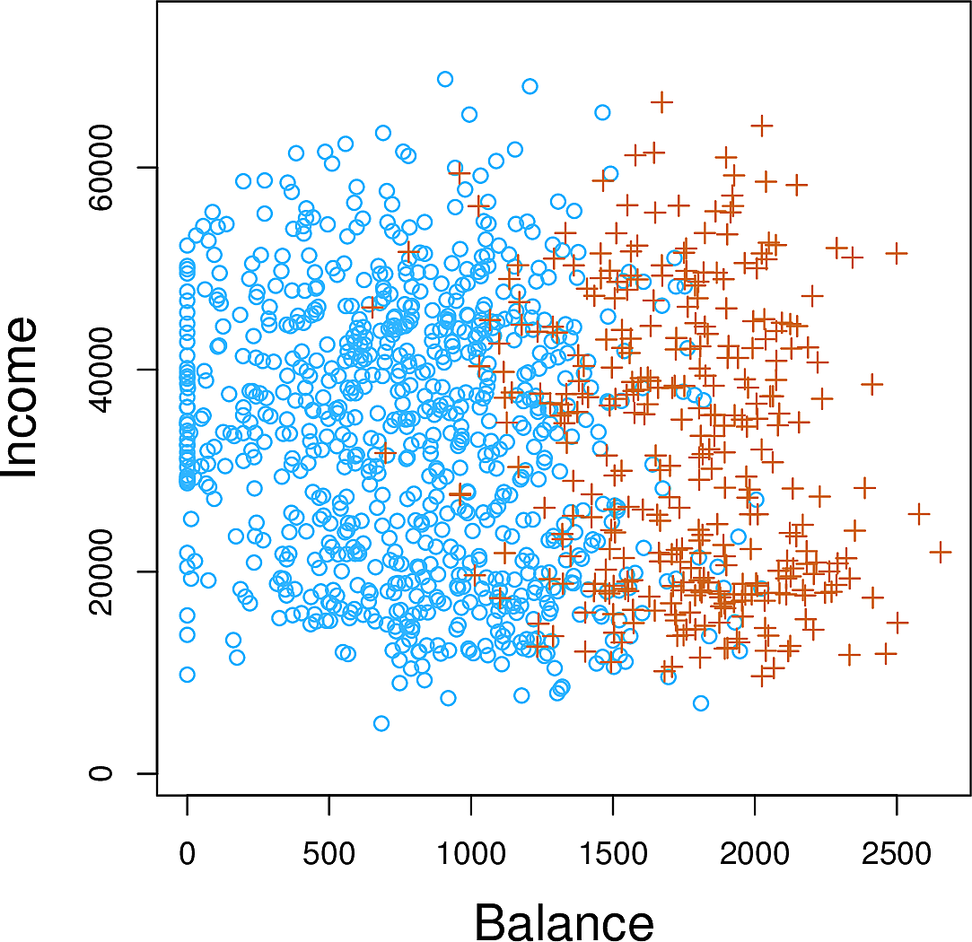
Let's look at the Default data set which aims to predict whether a credit card holder will default on their debt based on their monthly income and current credit card balance.

In this plot we show those who defaulted as orange pluses while those who did not as blue circles. The default rate is around 3% so the number of observations shown has been undersampled.

It appears that the defaults tend to have higher credit card balances.

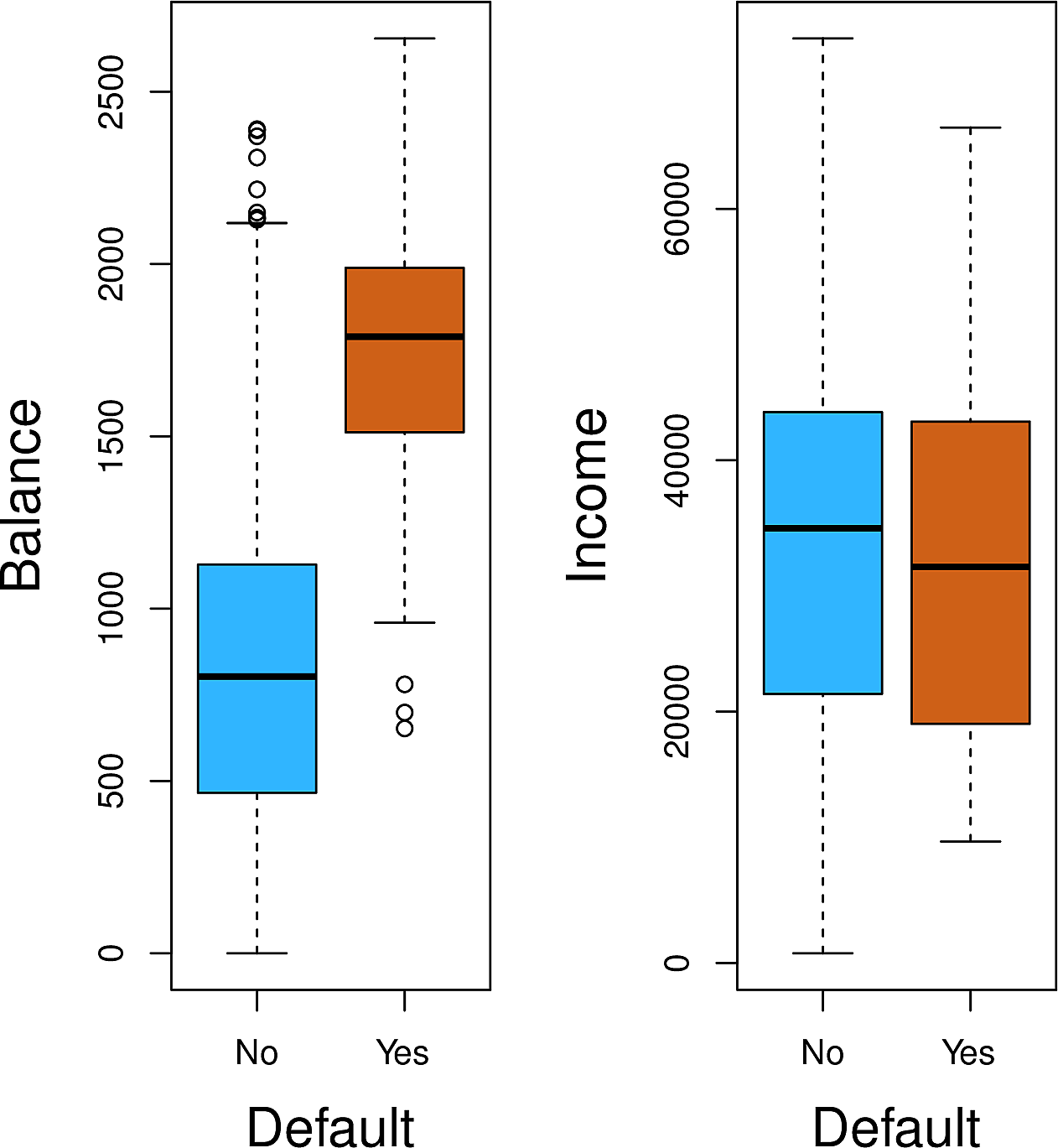
These boxplots show income and balance split by default. It appears that default has a strong relationship with balance but less so with income

Why not Linear Regression?

Consider a case where we would like to predict the medical condition of a patient in an emergency room. There are three possibilities: stroke, drug overdose and epileptic seizure? Couldn't we just encode these possibilities as numbers and do linear regression?

`stroke`	1
`drug overdose`	2
`epileptic seizure`	3

With the known interpretation of these numbers, this suggests that

drug overdose is in some sense between stroke and epileptic seizure
the "distance" between stroke and drug overdose is the same as that between drug overdose and epileptic seizure

Further if we had encoded them as follows

`epileptic seizure`	1
`stroke`	2
`drug overdose`	3

then we might get a different set of predictions.

We might use linear regression if there were some implied order between the categories, for example mild, moderate and severe, but still we are implying that the distance between mild and moderate is the same at that between moderate and severe.

For binary classification we could use the dummy variable approach to assign the values 0 and 1 to the two classes. For example:

\begin{equation} Y = \begin{cases} 0 & \text{if stroke} \\ 1 & \text{if drug overdose} \end{cases} \end{equation}

Now if our linear regression gives $\hat{Y} > 0.5$ we predict drug overdose or otherwise stroke. We can show that $\hat{Y}$ is an estimate for $P(\mathtt{drug overdose} | X)$.

But what if we get values for $\hat{Y}$ outside the $[0,1]$ interval? We can't interpret that as a probability!

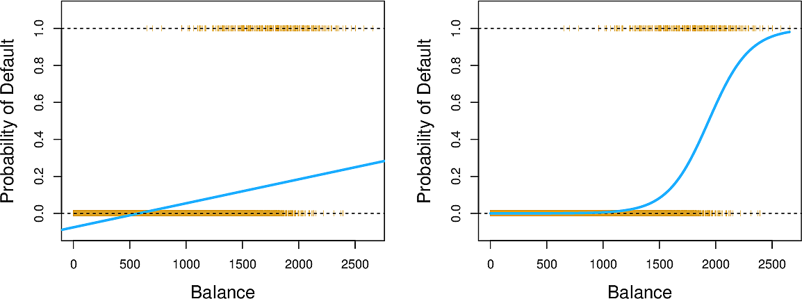
The blue line in the plot on the left is a linear regression for Default against Balance. Note how it takes negative values and always remains under $0.5$, suggesting that nobody will ever default. We now look into a technique which can transform this line into the blue line in the plot on the right, giving us interpretable probabilities.

Logistic regression

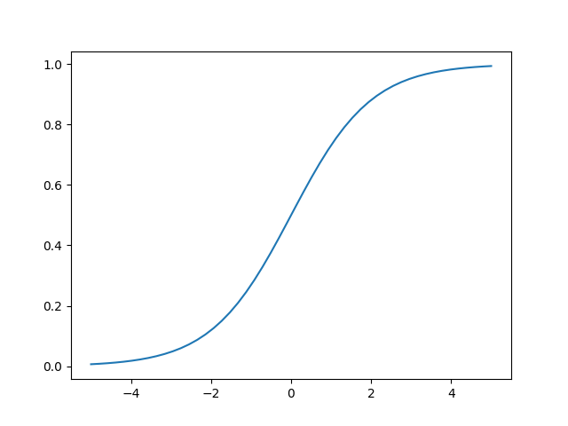
This is the logistic funciton. It has many applications in biology (especially ecology), biomathematics, chemistry, demography, economics, geoscience, mathematical psychology, probability, sociology, political science, linguistics, statistics, and even neural networks. \[ f(x) = \frac{1}{1 + e^{-x}} \]

import numpy as np
import matplotlib

# matplotlib.use("Agg")
import matplotlib.pyplot as plt


def logistic(x):
    return 1 / (1 + np.exp(-x))


# fig = plt.figure(figsize=(4, 2))
fig = plt.figure()
x = np.linspace(-5, 5)
plt.plot(x, logistic(x))
plt.savefig("images/python-matplot-fig.png")
plt.show()

Since this is a binary classification problem, to model the response directly we should predict whether Default is Yes or No. But we will take a different approach. We will model the probability that Default is Yes. We will write the probability that Default is Yes given a particular balance as \[ Pr(\mathtt{Default} = \mathtt{Yes} | \mathtt{balance}) \] We will abbreviate this as $p(\mathtt{balance})$.

We can choose our threshold. For example we can predict $\mathtt{Default} = \mathtt{Yes}$ whenever $p(\mathtt{balance}) > 0.5$ or whenever $p(\mathtt{balance}) > 0.1$

Now we can model $p_l$ as a straightforward linear regression problem: \[ p_l(X) = \beta_0 + \beta_1 X \]

But this could lead to the issue in the plot on the left above where we could get values less than zero or even greater than one.

So, instead of modelling $p_l(X)$, we will model $p(x) = f(p_l(X))$ where $f$ is the logistic function.

\[ p(X) = \frac{1}{1 + e^{-(\beta_0 + \beta_1 X)}} \]

The result of this is shown in the right plot above.

With a little algebra we can write \[ \frac{p(X)}{1-p(X)} = e^{\beta_0 + \beta_1 X} \] This quantity is called the odds. It can take any value in $[0,\inf)$

If one in five people default, then the odds will be \[ \frac{1/5}{1 - 1/5} = \frac{1}{4} \]

If nine out of ten people default, then the odds will be \[ \frac{9/10}{1 - 9/10} = 9 \]

If we take logarithms of both sides above we get \[ \log\left(\frac{p(X)}{1-p(X)}\right) = \beta_0 + \beta_1 X \]

This quantity is called the log odds or logit. Since the odds can take any value in $[0,\inf)$, the logit can take any value in $(-\inf, \inf)$.

We see that this logistic regression model has a logit linear in $X$. Increasing $X$ by one unit increases the log odds by $\beta_1$ and thus increases the odds by $e^\beta_1$.

Previously we used the method of least squares for linear regression. For logistic regression we will use a more general method called maximum likelihood.

The idea is this. We would like to predict a number as close as possible to $1$ for each credit card holder who defaulted and a number as close as possible to $0$ for each credit card holder who did not default.

We write $i:y_i=1$ for the set of indexes of those who defaulted and $i:y_i=0$ for those that did not. Now we write $\prod_{i:y_i=1} p(x_i)$ for the product of the probabilities of all those that defaulted and $\prod_{i:y_i=0} 1 - p(x_i)$ for the product of the probabilities of all those that did not default.

Now we write our likelihood function as a product of these \[ \mathcal{l}(\beta_0, \beta_1) = \prod_{i:y_i=1} p(x_i) \prod_{i:y_i=0} 1 - p(x_i) \]

Now we need to maximize this function to find $\hat\beta_0$ and $\hat\beta_1$.

Maximum likelihood estimation is an entire field in its own right. We will not be delving further into the theory in this course but let's look at how we can use it in practice.

Stock market data

Let's look at the Smarket data set which contains daily percentage returns for the S&P 500 stock index between 2001 and 2005.

First some imports

import statsmodels.api as sm
from ISLP import load_data
from ISLP.models import ModelSpec as MS

Now load the data and examine it.

Smarket = load_data("Smarket")
print(Smarket.shape)

(1250, 9)

print(Smarket.columns)

Index(['Year', 'Lag1', 'Lag2', 'Lag3', 'Lag4', 'Lag5', 'Volume', 'Today',
       'Direction'],
      dtype='object')

print(Smarket.describe())

              Year         Lag1         Lag2         Lag3         Lag4  \
count  1250.000000  1250.000000  1250.000000  1250.000000  1250.000000   
mean   2003.016000     0.003834     0.003919     0.001716     0.001636   
std       1.409018     1.136299     1.136280     1.138703     1.138774   
min    2001.000000    -4.922000    -4.922000    -4.922000    -4.922000   
25%    2002.000000    -0.639500    -0.639500    -0.640000    -0.640000   
50%    2003.000000     0.039000     0.039000     0.038500     0.038500   
75%    2004.000000     0.596750     0.596750     0.596750     0.596750   
max    2005.000000     5.733000     5.733000     5.733000     5.733000   

             Lag5       Volume        Today  
count  1250.00000  1250.000000  1250.000000  
mean      0.00561     1.478305     0.003138  
std       1.14755     0.360357     1.136334  
min      -4.92200     0.356070    -4.922000  
25%      -0.64000     1.257400    -0.639500  
50%       0.03850     1.422950     0.038500  
75%       0.59700     1.641675     0.596750  
max       5.73300     3.152470     5.733000

Smarket.corr(numeric_only=True)

Let's look at the market Volume by day.

print(Smarket.plot(y="Volume"))

We now fit a logistic regression model to predict the categorical variable Direction to Volume and the lag columns. We would like to predict whether the market will go Up or Down based on its behaviour over the previous five days.

Since logistic regression is a special case of the more general Generalized Linear Models we use GLM with the Binomial family of distributions.

df_lagvol = Smarket.columns.drop(["Today", "Direction", "Year"])
design = MS(df_lagvol)
X = design.fit_transform(Smarket)
y = Smarket.Direction == "Up"
logreg = sm.GLM(y, X, family=sm.families.Binomial())
results = logreg.fit()
print(results.summary())

                 Generalized Linear Model Regression Results                  
==============================================================================
Dep. Variable:              Direction   No. Observations:                 1250
Model:                            GLM   Df Residuals:                     1243
Model Family:                Binomial   Df Model:                            6
Link Function:                  Logit   Scale:                          1.0000
Method:                          IRLS   Log-Likelihood:                -863.79
Date:                Mon, 06 Oct 2025   Deviance:                       1727.6
Time:                        12:56:39   Pearson chi2:                 1.25e+03
No. Iterations:                     4   Pseudo R-squ. (CS):           0.002868
Covariance Type:            nonrobust                                         
==============================================================================
                 coef    std err          z      P>|z|      [0.025      0.975]
------------------------------------------------------------------------------
intercept     -0.1260      0.241     -0.523      0.601      -0.598       0.346
Lag1          -0.0731      0.050     -1.457      0.145      -0.171       0.025
Lag2          -0.0423      0.050     -0.845      0.398      -0.140       0.056
Lag3           0.0111      0.050      0.222      0.824      -0.087       0.109
Lag4           0.0094      0.050      0.187      0.851      -0.089       0.107
Lag5           0.0103      0.050      0.208      0.835      -0.087       0.107
Volume         0.1354      0.158      0.855      0.392      -0.175       0.446
==============================================================================

In particular we look at the $p$-values

print(results.pvalues)

intercept    0.600700
Lag1         0.145232
Lag2         0.398352
Lag3         0.824334
Lag4         0.851445
Lag5         0.834998
Volume       0.392404
dtype: float64

None of them is particularly small. This is unsurprising; if we could predict market behaviour from previous days' performance we could make a lot of money!

Predicting credit-card defaults

Now let's return to the credit card data set and predict Default from balance.

df_cc = load_data('Default')
print(df_cc.shape)

(10000, 4)

print(df_cc.columns)

Index(['default', 'student', 'balance', 'income'], dtype='object')

print(df_cc)

     default student      balance        income
0         No      No   729.526495  44361.625074
1         No     Yes   817.180407  12106.134700
2         No      No  1073.549164  31767.138947
3         No      No   529.250605  35704.493935
4         No      No   785.655883  38463.495879
...      ...     ...          ...           ...
9995      No      No   711.555020  52992.378914
9996      No      No   757.962918  19660.721768
9997      No      No   845.411989  58636.156984
9998      No      No  1569.009053  36669.112365
9999      No     Yes   200.922183  16862.952321

[10000 rows x 4 columns]

df_balance = df_cc[["balance"]]
design = MS(df_balance)
X = design.fit_transform(df_cc)
y = df_cc.default == "Yes"
logreg = sm.GLM(y, X, family=sm.families.Binomial())
results = logreg.fit()
print(results.summary())

                 Generalized Linear Model Regression Results                  
==============================================================================
Dep. Variable:                default   No. Observations:                10000
Model:                            GLM   Df Residuals:                     9998
Model Family:                Binomial   Df Model:                            1
Link Function:                  Logit   Scale:                          1.0000
Method:                          IRLS   Log-Likelihood:                -798.23
Date:                Mon, 06 Oct 2025   Deviance:                       1596.5
Time:                        12:56:39   Pearson chi2:                 7.15e+03
No. Iterations:                     9   Pseudo R-squ. (CS):             0.1240
Covariance Type:            nonrobust                                         
==============================================================================
                 coef    std err          z      P>|z|      [0.025      0.975]
------------------------------------------------------------------------------
intercept    -10.6513      0.361    -29.491      0.000     -11.359      -9.943
balance        0.0055      0.000     24.952      0.000       0.005       0.006
==============================================================================

Let's have a look at some of the predictions for the training set.

print(results.predict()[:8])

[0.00130568 0.00211259 0.00859474 0.00043444 0.00177696 0.00370415
 0.00221143 0.00201617]

We convert these probabilities into labels Yes or No

labels = np.array(['No '] * df_cc.shape[0])
labels[results.predict() > 0.5] = 'Yes'
print(np.unique(labels, return_counts=True))

(array(['No ', 'Yes'], dtype='<U3'), array([9858,  142]))

Now let's make predictions for the probabilities of default for credit-card holders with balances of $1000 and $2000.

df_new = pd.DataFrame({"balance": [1000, 2000]})
X_new = design.transform(df_new)
predictions = results.get_prediction(X_new)
print(predictions.predicted_mean)

---------------------------------------------------------------------------
NameError                                 Traceback (most recent call last)
Cell In[14], line 1
----> 1 df_new = pd.DataFrame({"balance": [1000, 2000]})
      2 X_new = design.transform(df_new)
      3 predictions = results.get_prediction(X_new)

NameError: name 'pd' is not defined

We map these probabilities to labels.

label = np.vectorize(lambda x: 'Yes' if x > 0.5 else 'No')
print(label(predictions.predicted_mean))

---------------------------------------------------------------------------
NameError                                 Traceback (most recent call last)
Cell In[15], line 2
      1 label = np.vectorize(lambda x: 'Yes' if x > 0.5 else 'No')
----> 2 print(label(predictions.predicted_mean))

NameError: name 'predictions' is not defined

We see that the model predicts that a credit-card holder with a balance of $1000 has less than half a percent probability to default while one with a balance of $2000 has nearly a 60% probability to default.

To use these probabilities for a classification task we could assign a Default of Yes to any credit-card holder with a greater that 50% probability and No otherwise.

However note that although we get numbers between 0 and 1, these are not necessarily "probabilities" in the true sense of the word. As such we can choose another threshold than $0.5$, perhaps $0.6$ if it gives us better predictions. This may help in a case like this were we have highly imbalanced data with only about 3% of the data points having a Default of Yes.

etc

Note that there is an errata page for the book
Python f-string cheat sheets
Feedback on the Linear Regression assignment

The week's teams

[('Adrian', 'Emil'),
 ('Jess', 'Janina'),
 ('Carlijn', 'Fridolin'),
 ('Asmahene', 'Jagoda'),
 ('Efraim', 'Lynn'),
 ('Romane', 'Natalia'),
 ('Henrike', 'Giorgia'),
 ('Matúš', 'Madalina'),
 ('Yaohong', 'Max'),
 ('Nora', 'Mariana'),
 ('Emilio', 'Louanne', 'Roman'),
 ]