Course Introduction
Today
- Getting to know each other
- Housekeeping: book, assignments, exams, grading, expectations
- What is Machine Learning?
- Some history
- ML around us today and its effects on our lives
Machine Learning
Machine Learning is the field of study that gives computers the ability to learn without being explicitly programmed.
– Arthur Samuel, 1959
Machine Learning is the science (and art) of programming computers so they can learn from data.
– Aurélien Géron
A computer program is said to learn from experience E with respect to some class of tasks T, and performance measure P, if its performance at tasks in T, as measured by P, improves with experience E.
– Tom Mitchell
Probabilistic reasoning
We will treat all unknown quantities as random variables, that are endowed with probability distributions which describe a weighted set of possible values the variable may have.
Almost all of machine learning can be viewed in probabilistic terms, making probabilistic thinking fundamental. It is, of course, not the only view. But it is through this view that we can connect what we do in machine learning to every other computational science, whether that be in stochastic optimisation, control theory, operations research, econometrics, information theory, statistical physics or bio-statistics. For this reason alone, mastery of probabilistic thinking is essential.
– Shakir Mohamed, DeepMind
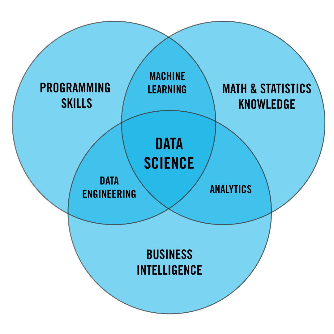
Data Science
An example: Spam filtering
- spam, ham
- training set of training instances
- performance measure: ratio of correctly classified emails: accuracy.
- How would you write a program to detect spam?
- "Typical" spam
- Patterns
- Test and tune
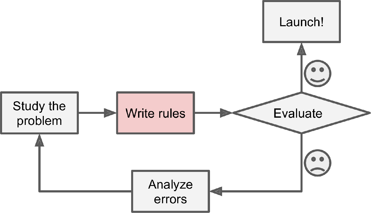
Figure 1: A traditional approach
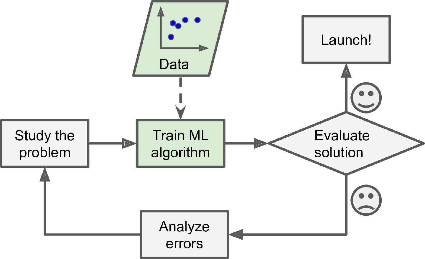
Figure 2: A Machine Learning approach
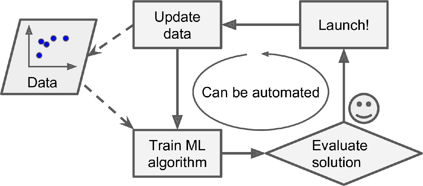
Figure 3: Adapting to change
An Interactive Introduction to Machine Learning


Identifying flowers
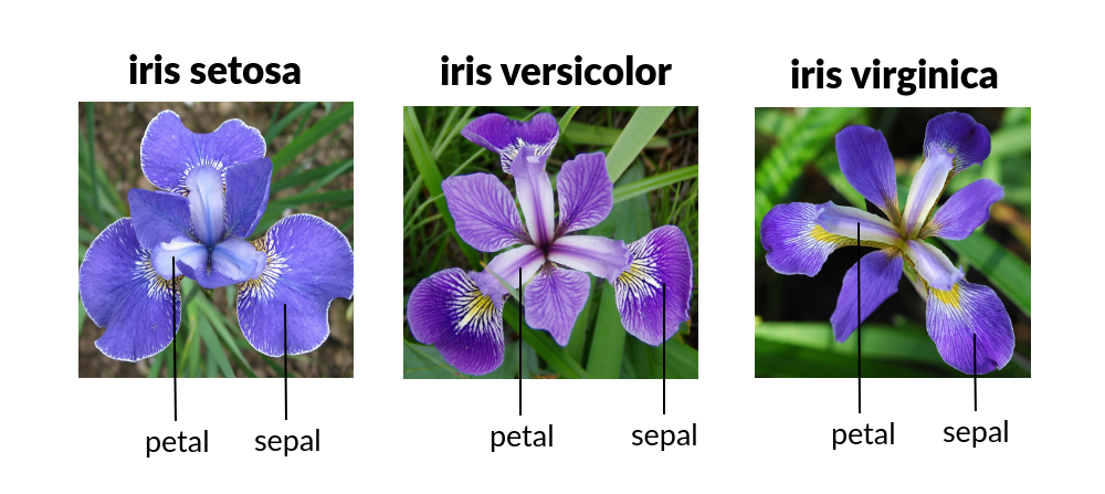
import polars as pl

iris_file = "https://ml.auc-computing.nl/data/iris.csv"

df = pl.read_csv(iris_file)
df
| 150 | 4 | setosa | versicolor | virginica |
|---|---|---|---|---|
| f64 | f64 | f64 | f64 | i64 |
| 5.1 | 3.5 | 1.4 | 0.2 | 0 |
| 4.9 | 3.0 | 1.4 | 0.2 | 0 |
| 4.7 | 3.2 | 1.3 | 0.2 | 0 |
| 4.6 | 3.1 | 1.5 | 0.2 | 0 |
| 5.0 | 3.6 | 1.4 | 0.2 | 0 |
| … | … | … | … | … |
| 6.7 | 3.0 | 5.2 | 2.3 | 2 |
| 6.3 | 2.5 | 5.0 | 1.9 | 2 |
| 6.5 | 3.0 | 5.2 | 2.0 | 2 |
| 6.2 | 3.4 | 5.4 | 2.3 | 2 |
| 5.9 | 3.0 | 5.1 | 1.8 | 2 |
df = pl.read_csv(
    iris_file,
    has_header=True,
    new_columns=[
        "sepal_length",
        "sepal_width",
        "petal_length",
        "petal_width",
        "class_id",
    ],
)

df_head = pl.read_csv(
    iris_file,
    has_header=True,
    n_rows=0
)
species = df_head.columns[2:]
mapping = pl.DataFrame(
    {"class_id": list(range(len(species))), "species": species}
)
df = df.join(mapping, on="class_id")
df
| sepal_length | sepal_width | petal_length | petal_width | class_id | species |
|---|---|---|---|---|---|
| f64 | f64 | f64 | f64 | i64 | str |
| 5.1 | 3.5 | 1.4 | 0.2 | 0 | "setosa" |
| 4.9 | 3.0 | 1.4 | 0.2 | 0 | "setosa" |
| 4.7 | 3.2 | 1.3 | 0.2 | 0 | "setosa" |
| 4.6 | 3.1 | 1.5 | 0.2 | 0 | "setosa" |
| 5.0 | 3.6 | 1.4 | 0.2 | 0 | "setosa" |
| … | … | … | … | … | … |
| 6.7 | 3.0 | 5.2 | 2.3 | 2 | "virginica" |
| 6.3 | 2.5 | 5.0 | 1.9 | 2 | "virginica" |
| 6.5 | 3.0 | 5.2 | 2.0 | 2 | "virginica" |
| 6.2 | 3.4 | 5.4 | 2.3 | 2 | "virginica" |
| 5.9 | 3.0 | 5.1 | 1.8 | 2 | "virginica" |
df.group_by("species").len()
| species | len |
|---|---|
| str | u32 |
| "setosa" | 50 |
| "virginica" | 50 |
| "versicolor" | 50 |
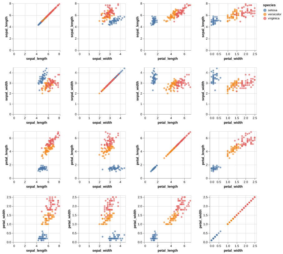
import altair as alt

adf = df.drop("class_id")
features = adf.drop('species').columns

alt.Chart(adf).mark_circle().encode(
    alt.X(alt.repeat("column"), type="quantitative"),
    alt.Y(alt.repeat("row"), type="quantitative"),
    color="species:N",
).properties(width=150, height=150).repeat(
    row=features, column=features,
).save('images/iris_altair_pairplot.png')
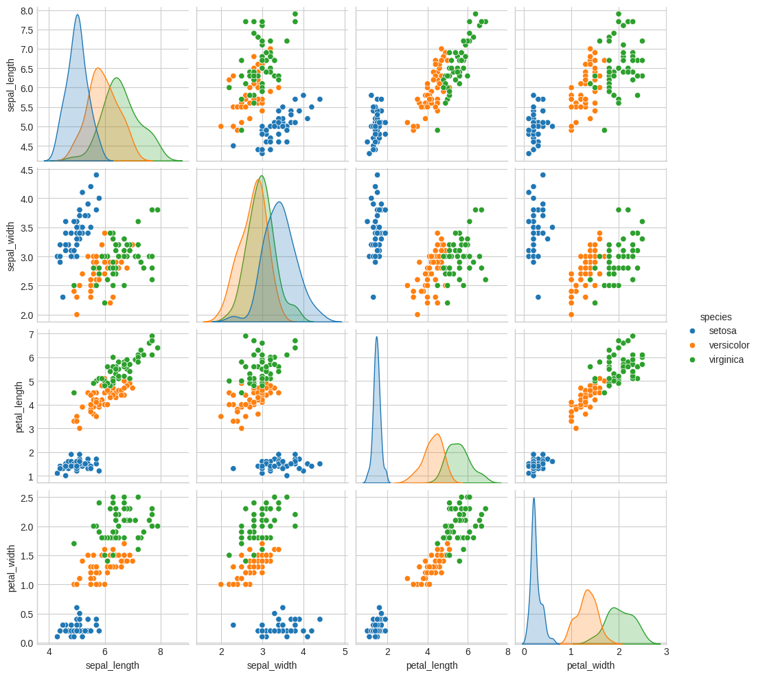
import seaborn as sns

pdf = df.drop('class_id').to_pandas()

sns.pairplot(pdf, hue="species").savefig("images/iris_pairplot.png")
- data frame
- design matrix
- tabular data
- features and target
- supervised learning
- classification
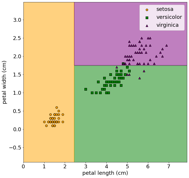


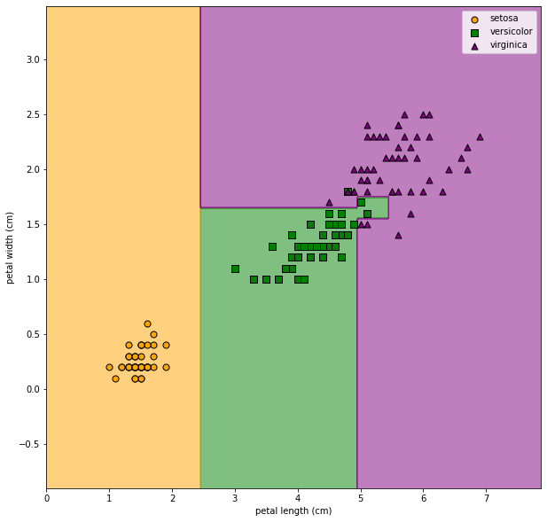
- Misclassification rate
- Asymmetric loss matrix
| Setosa | Versicolor | Virginia | |
|---|---|---|---|
| Setosa | 0 | 1 | 1 |
| Versicolor | 1 | 0 | 1 |
| Virginia | 10 | 10 | 0 |
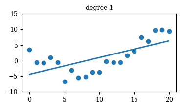
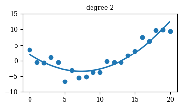
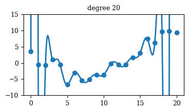
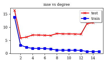
Regression


Mastering Data
- Information for humans and information for programs
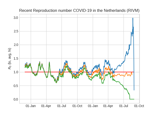
- Dutch National Institute for Public Health and the Environment
# Download latest RIVM data on R_0 and plot it.

from requests import get
import pandas as pd
import numpy as np
import matplotlib.pyplot as plt
from matplotlib import dates as mpl_dates
from datetime import datetime, timedelta

plt.style.use("seaborn-v0_8-whitegrid")
# plt.style.use("seaborn-v0_8-darkgrid")

date_format = mpl_dates.DateFormatter("%d-%b")
plt.gca().xaxis.set_major_formatter(date_format)

w = get("https://data.rivm.nl/covid-19/COVID-19_reproductiegetal.json")
days = w.json()


def plot_key(key):
    key_by_day = [
        float(day[key]) if key in day and day[key] else np.nan for day in days
    ]
    day_count = len(key_by_day)
    start_date = datetime.today() - timedelta(day_count)
    dates = pd.date_range(start_date, periods=day_count)

    plt.plot_date(dates, key_by_day, "-")


day_count = len(days)
start_date = datetime.today() - timedelta(day_count)
all_dates = pd.date_range(start_date, periods=day_count)
plt.plot_date(all_dates, [1.0] * day_count, "r-")

plot_key("Rt_up")
plot_key("Rt_avg")
plot_key("Rt_low")

plt.title("Recent Reproduction number COVID-19 in the Netherlands (RIVM)")
plt.ylabel("$R_0$ (lo, avg, hi)")

plt.savefig("images/r0.png")
# plt.show()
- Getting tables from HTML pages. Suppose we are interested in Gini coefficients for countries.
from requests import get
import pandas as pd
from io import StringIO

url = "https://en.wikipedia.org/wiki/List_of_countries_by_income_equality"
header = {
    "User-Agent": (
        "Mozilla/5.0 (X11; Linux x86_64) AppleWebKit/537.36 "
        "(KHTML, like Gecko) Chrome/50.0.2661.75 Safari/537.36"
    ),
    "X-Requested-With": "XMLHttpRequest",
}

r = get(url, headers=header)

pdf = pd.read_html(StringIO(r.text))[0]
gini_table = pl.from_pandas(pdf)
gini_table
| ('Country/Territory', 'Country/Territory') | ('UN Region', 'UN Region') | ('World Bank Income group (2024)', 'World Bank Income group (2024)') | ('Gini coefficient[a]', 'WB[2]') | ('Gini coefficient[a]', 'Year') | ('Gini coefficient[a]', 'UNU- WIDER[3]') | ('Gini coefficient[a]', 'Year.1') | ('Gini coefficient[a]', 'OECD[4][5][6]') | ('Gini coefficient[a]', 'Year.2') | ('Unnamed: 9_level_0', 'Unnamed: 9_level_1') |
|---|---|---|---|---|---|---|---|---|---|
| str | str | str | str | str | str | str | str | str | str |
| "Afghanistan" | "Southern Asia" | "Low income" | null | null | "31.00" | "2017" | null | null | null |
| "Angola" | "Middle Africa" | "Lower middle income" | "51.3" | "2018" | "51.27" | "2019" | null | null | null |
| "Albania" | "Southern Europe" | "Upper middle income" | "29.4" | "2020" | "29.42" | "2020" | null | null | null |
| "Andorra" | "Southern Europe" | "High income" | null | null | "27.96" | "2016" | null | null | null |
| "United Arab Emirates" | "Western Asia" | "High income" | "26.4" | "2018" | "25.97" | "2019" | null | null | null |
| … | … | … | … | … | … | … | … | … | … |
| "Yemen" | "Western Asia" | "Low income" | "36.7" | "2014" | "36.71" | "2014" | null | null | null |
| "South Africa" | "Southern Africa" | "Upper middle income" | "63.0" | "2014" | "66.99" | "2017" | null | null | null |
| "Zambia" | "Eastern Africa" | "Lower middle income" | "51.5" | "2022" | "44.00" | "2022" | null | null | null |
| "Zimbabwe" | "Eastern Africa" | "Lower middle income" | "50.3" | "2019" | "50.26" | "2019" | null | null | null |
| "^ The Gini coefficient, or Gin… | "^ The Gini coefficient, or Gin… | "^ The Gini coefficient, or Gin… | "^ The Gini coefficient, or Gin… | "^ The Gini coefficient, or Gin… | "^ The Gini coefficient, or Gin… | "^ The Gini coefficient, or Gin… | "^ The Gini coefficient, or Gin… | "^ The Gini coefficient, or Gin… | "^ The Gini coefficient, or Gin… |
Some History
- 1805
- Legendre developed Least Squares Linear Regression to predict the movement of the planets
- 1936
- Linear Discriminant Analysis was developed do predict qualitative results.
- 1940s
- Logistic Regression
- 1952
- Arthur Samuel develops the first computer program to play Checkers using the Minimax algorithm and coins the phrase "Machine Learning"
- 1957
- The Perceptron
- 1967
- The Nearest Neighbor Algorithm
- 1970s
- Generalized Linear Models
- 1980s
- Computing technology had evolved to the point where non-linear methods could be developed for
- 1990s
- Support Vector Machines
- 1997
- Schmidhuber and Hochreiter develop long short-term memory for speech recognition.
- 2006
- The Facial Recognition Grand Challenge shows significant progress
- 2013
- Atari games
Machine Learning today
- Self-driving cars
- Voice technologies: Siri, Alexa, etc
- Large Language Models: ChatGPT, LLaMA and many others
- “As soon as it works, no one calls it AI anymore.” – John McCarthy

- Google's latest smartphone model
- Ethical questions, data privacy and ownership, reward hacking and the alignment problem.
Course overview and housekeeping
Course home page
We do not put the course material on Canvas. Rather, we build a website in the course of the semester. Each class will have its own page which will contain links to all of the materials discussed.
Classes
- Monday: Lecture in 2.05, 15:45–17:30
- Thursday: Lab in 2.05, 11:00–12:45
- During lectures you will be presented with material on various topics in Machine learning. This will be mostly with closed laptops. You may find it useful to have pen and paper to take occasional notes.
- During the labs you will be working on material you have learned in the previous lecture. Make sure you have your laptop with the necessary software tools.
- Attendance will be taken at the beginning of each class. Please come on time. Late = absent.
Teacher
- Breanndán Ó Nualláin
<o@uva.nl>
Book
An Introduction to Statistical Learning by James, Witten, Hastie & Tibshirani. The full text is available from that link.
Assignments
- There will be one graded assignment. It will be an assignment on Data Ethics which you will carry out in groups of ±4. You will write a report and give a presentation on a topic of your choice. The deadline for submission of the report and presentation is the date of the presentations.
- Each Thursday you will be given an assignment consisting of a set of applied tasks. The goal is for you to familiarise yourself with the material covered in the Monday class by putting it into practice and submitting it during the Thursday lab class.
- Assignments will not be graded but students will receive feedback on their work.
- As each exam will be similar in form to one of these assignments, carrying out the assignments is essential to acquire then necessary knowledge and skills to take the exams.
- The first assignments will be in pairs. Later assignments will be individual.
Grading
See the section on Assessment in the Course manual.
Programming environment
In this course we will emphasise good programming practice by using professional software tools and methods. In particular note that the book recommends using Jupyter. However we will not be using Jupyter in this course. For programming you may use Spyder or one of a range of other IDEs.
My own preferred development environment is Emacs, a highly flexible and powerful tool which has an intimidating learning curve. During the course, I will show you how to use Emacs but you are not required to learn it.
Why not Jupyter?
Software tools
Since we will be working with large data sets we will learn to use professional tools for programming and managing the software that we develop. Among these are:
- Python
- Some Python libraries:
- Numpy adds support for large, multi-dimensional arrays and matrices, along with a large collection of high-level mathematical functions to operate on these arrays.
- Pandas offers data structures and operations for manipulating numerical tables and time series.
- Polars coherent, fast, dataframes (lazy, column-oriented, out-of-memory).
- Scikit-learn features various classification, regression and clustering algorithms as well as tools for building powerful data pipelines.
- Matplotlib is a comprehensive library for creating static, animated, and interactive data visualizations in Python.
- Seaborn is a Python data visualization library based on matplotlib. It provides a high-level interface for drawing attractive and informative statistical graphics.
- Anaconda is a distribution of the Python programming language for scientific computing, containing the above libraries and more. It aims to simplify package management and deployment. Anaconda has questionable licensing terms that you might not like to agree to.
- Spyder is an Interactive Development Environment (IDE) for Python included in Anaconda
- Emacs is an extensible, customizable, free/libre text editor. It includes a full development environment for Python and interaction with Git and many other features.
- Git Git is a free and open source distributed version control system.
- Forgejo is a web-based collaborative software platform for both developing and sharing computer applications. AUC runs its own instance of Forgejo
Assignments
- In the labs you will work in pairs for the first few weeks.. Each week the pairs will be assigned randomly.
- You will receive an assignment to be worked on in class on Thursdays. Together with your partner, you can also work on the assignment before and after class.
- This coming Thursday we will set up our computational environment and software tools. This is very important because you will not be able to program or submit anything until you have them set up correctly.
- In the meantime you might like to read the introductory chapter of An Introduction to Statistical Learning